Before going to discuss how computer identifies and labels objects let’s understand what is computer vision in detail.
“Computer vision is the field of having a computer understand and label what is present in an image(i.e, this is a dog or cat without being explicitly programmed) and then figure out the patterns.”
You can interpret what a shirt is or what a shoe is, but how would you program for that? if an extra terrestrial who had never seen clothing walked into the room with you, how would you explain the shoes to him? It’s really difficult, if not impossible to do right? And it’s the same problem with computer vision.
So one way to solve that is to use lots of pictures of clothing and tell the computer what that’s a picture of and then have the computer figure out the patterns that give you the difference between a shoe, and a shirt, and a handbag, and a coat.
For example, take a computer vision problem? Let’s take a look at a scenario where we can recognize different items of clothing, trained from a data set containing 10 different types.
Fashion-MNIST is available as a data set with an API call in TensorFlow(Tensorflow has in-built data sets available for learning purposes we just need to import them) but before that let’s start with our import of TensorFlow.
import tensorflow as tf
print(tf.__version__)
The Fashion MNIST data is available directly in the tf.keras datasets API. You load it like below.
mnist = tf.keras.datasets.fashion_mnistIn the MNIST data set, 60,000 of the 70,000 images are used to train the network, and then 10,000 images, one that it hasn’t previously seen, can be used to test just how good or how bad it is performing.
Calling load_data on this object will give you two sets of two lists, these will be the training and testing values for the graphics that contain the clothing items and their labels.
(training_images, training_labels), (test_images, test_labels) = mnist.load_data()What do these values look like? Let’s print a training image, and a training label to see…Experiment with different indices in the array. For example, also take a look at index 0.
import numpy as np
np.set_printoptions(linewidth=200)
import matplotlib.pyplot as plt
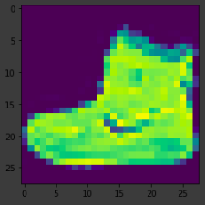
plt.imshow(training_images[0])
print(training_labels[0])
print(training_images[0])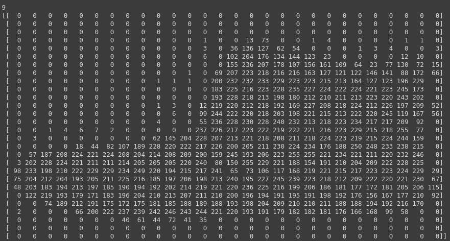
If you notice that all of the values in the number are between 0 and 255. If we are training a neural network, for various reasons it’s easier if we treat all values as between 0 and 1, a process called ‘normalizing‘…and fortunately in Python it’s easy to normalize a list like this without looping.
training_images  = training_images / 255.0
test_images = test_images / 255.0
Now you might be wondering why there are 2 sets…training and testing — remember the idea is to have 1 set of data for training, and then another set of data for testing…that the model hasn’t yet seen…to see how good it would be at classifying values. After all, when you’re done, you’re going to want to try it out with data that it hadn’t previously seen!
Let’s now design the model. There are quite a few new concepts here but don’t worry, you’ll get the hang of them by reading the description below.
model = tf.keras.models.Sequential([tf.keras.layers.Flatten(),
                                    tf.keras.layers.Dense(128, activation=tf.nn.relu),
tf.keras.layers.Dense(10, activation=tf.nn.softmax)])Sequential: That defines a SEQUENCE of layers in the neural network.
Flatten: Remember earlier where our images were a square when you printed them out? Flatten just takes that square and turns it into a 1-dimensional set.
Dense: Adds a layer of neurons.
Each layer of neurons needs an activation function to tell them what to do. There are lots of options, but just use these for now.
Relu effectively means “If X>0 return X, else return 0” — so what it does it only passes values 0 or greater to the next layer in the network.
Softmax takes a set of values, and effectively picks the biggest one, so, for example, if the output of the last layer looks like [0.1, 0.1, 0.05, 0.1, 9.5, 0.1, 0.05, 0.05, 0.05], it saves you from fishing through it looking for the biggest value, and turns it into [0,0,0,0,1,0,0,0,0] — The goal is to save a lot of coding! as well as time.
The next thing to do, now the model is defined, is to actually build it. You do this by compiling it with an optimizer and loss function as before — and then you train it by calling *model.fit * asking it to fit your training data to your training labels — i.e. have it figure out the relationship between the training data and its actual labels, so in future, if you have data that looks like the training data, then it can make a prediction for what that data would look like.
model.compile(optimizer = tf.optimizers.Adam(),
              loss = 'sparse_categorical_crossentropy',
              metrics=['accuracy'])

model.fit(training_images, training_labels, epochs=5)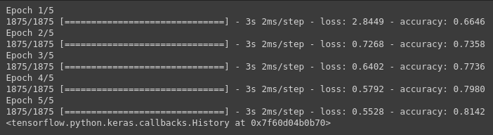
Once it’s done training — you should see an accuracy value at the end of the final epoch. It might look something like 0.8142. This tells you that your neural network is about 81% accurate in classifying the training data. I.E., it figured out a pattern match between the image and the labels that worked 81% of the time. Not great, but not bad considering it was only trained for 5 epochs and done quite quickly.
But how would it work with unseen data? That’s why we have the test images.
We can call the function model.evaluate, and pass in the two sets, and it will report back the loss for each. Let’s take a look.
model.evaluate(test_images, test_labels)
An accuracy that was returned was about .7971, which means it was about 79% accurate. As expected it probably would not do as well with unseen data as it did with data it was trained on! As we move further, there are ways to improve this.
To explore further, let’s create a set of classifications for each of the test images, and then prints the first entry in the classifications.
classifications = model.predict(test_images)

print(classifications[0])
[8.9938662e-10, 1.9189129e-05, 1.6107211e-19, 4.0872710e-09, 2.3770831e-16, 1.9478011e-01, 4.6645251e-13, 1.3415834e-01, 5.3518648e-05, 6.7098886e-01]
The output of the model is a list of 10 numbers. These numbers are a probability that the value being classified is the corresponding value, i.e., the first value in the list is the probability that the image is of a ‘0’ (T-shirt/top), the next is a ‘1’ (Trouser), etc. Notice that they are all VERY LOW probabilities.
For the 9 (Ankle boot), the probability was in the ’90s, i.e. the neural network is telling us that it’s almost certainly a 7. The 10th element on the list is the biggest, and the ankle boot is labeled 9. The list has the 10th element being the highest value means that the Neural Network has predicted that the item it is classifying is most likely an ankle boot.
We came to the end, so far we have loaded data, built a model, and fed with training data we predicted ankle boot. A few key points to consider are:
Increase the number of neurons — The impact is training takes longer but results are accurate. By adding more Neurons we have to do more calculations, slowing down the process, but in this case, they have a good impact — we do get more accurate. That doesn’t mean it’s always a case of ‘more is better’, you can hit the law of diminishing returns very quickly!
Remove the Flatten() layer. Why do you think that’s the case you get an error about the shape of the data. It may seem vague right now, but it reinforces the rule of thumb that the first layer in your network should be the same shape as your data. Right now our data is 28×28 images, and 28 layers of 28 neurons would be infeasible, so it makes more sense to ‘flatten’ that 28,28 into a 784×1. Instead of writing all the code to handle that ourselves, we add the Flatten() layer at the beginning, and when the arrays are loaded into the model later, they’ll automatically be flattened for us.
Change final (output) layers — You get an error as soon as it finds an unexpected value. Another rule of thumb — the number of neurons in the last layer should match the number of classes you are classifying for. In this case, it’s the digits 0-9, so there are 10 of them, hence you should have 10 neurons in your final layer.
Consider the effects of additional layers in the network — There isn’t a significant impact — because this is relatively simple data. For far more complex data (including color images to be classified as flowers), extra layers are often necessary.
The impact of training for more or fewer epochs — you might see the loss value stops decreasing, and sometimes increases. This is a side effect of something called ‘over-fitting’ and you need to keep an eye out for when training neural networks. There’s no point in wasting your time training if you aren’t improving your loss, right!
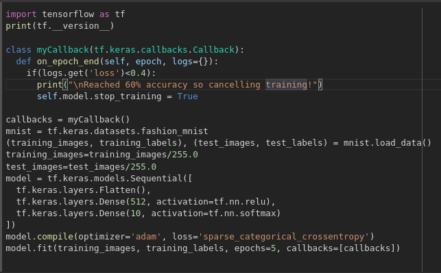
Callbacks — stop the training when I reach the desired value?’ — i.e. 95% accuracy might be enough for you, and if you reach that after 3 epochs, why sit around waiting for it to finish a lot more epochs…So how would you fix that? Like any other program…you have callbacks! Let’s see them in action…
Still, have any doubts? feel free to contact us.