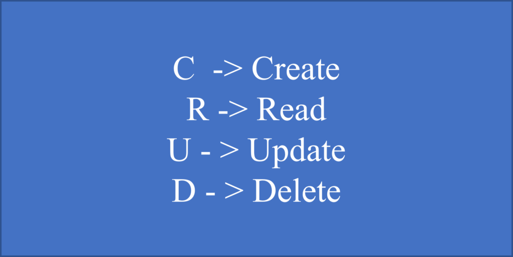
CRUD is an acronym that stands for Create, Read, Update and Delete.
Each letter in acronym refers to all functions executed in a database and mapped to standard HTTP method, SQL statement. CRUD is data-oriented and standardized use of HTTP action methods. This consists of four basic operations which we can perform in a Database table.
Each letter in CRUD corresponds to HTTP request method.
Create –> POST
Read –> GET
Update –> PUT or PATCH
Delete –> DELETE
Create:
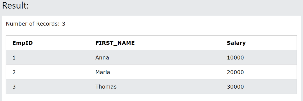
Create means to add or insert data into the table. First we will create table using CREATE TABLE command and then add data using INSERT INTO command.
SQL Command to create table:
CREATE TABLE employee(EmpID int PRIMARY KEY, FIRST_NAME VARCHAR, Salary INT);
Read means retrieving or fetching data or information from the table. We will use SELECT command to fetch data from the table. There is also an option of retrieving only those records which satisfy a particular condition by using the WHERE clause in a SELECT query.
SQL command to fetch data:
SELECT *from employee;
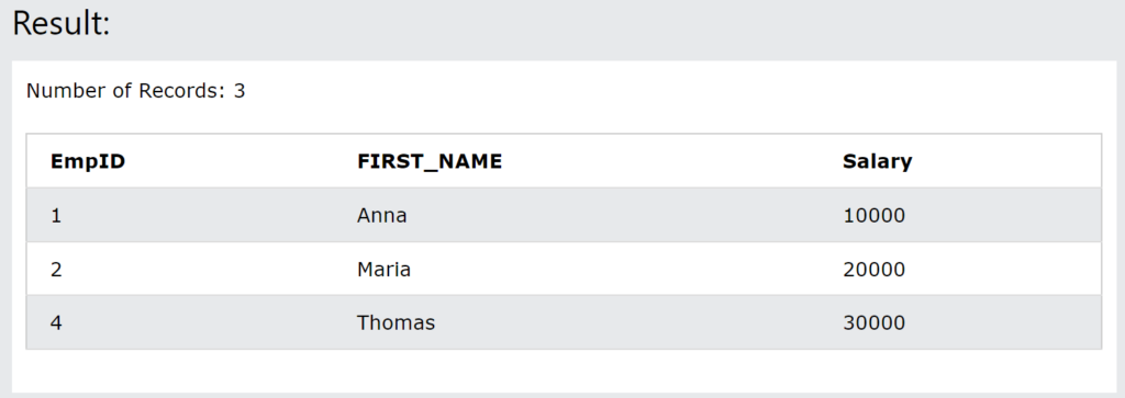
Update:
Update operation makes changes in the table by modifying the data. We will use UPDATE command to make changes in the data present in tables.
SQL command to Update records:
Update employee SET EmpID = 4 WHERE First_Name = ‘Thomas’;
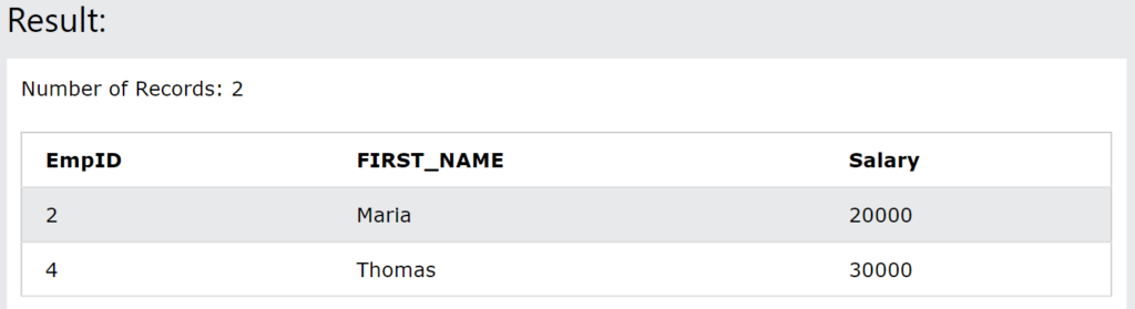
Delete:
Delete operation deletes the records from table. We can delete all the rows or a particular row using DELETE query.
SQL command to delete records:
DELETE FROM employee where Salary = 10000;
These are the basic CRUD operations in SQL. We also have another article about CRUD operation in Python. If you are interested you can go and check the article.
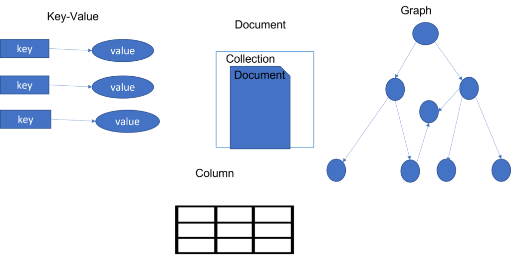
In the above images we can understand the models of SQL and NoSQL databases.
If your application has fixed structure and does not require frequent modifications then SQL is best. But if your application is rapidly changing and growing like in big data analytics then NoSQL is best.
In this article. we’ll discuss AI in detail, and talk about Components of AI and Use Cases, applications of AI in real-world.
Al refers to the ability of machines to perceive, learn, interact with the environment, analyze, and solve problems independently.
Let us take a closer look at how Al-driven systems interact with our environment. Like us humans, Al-driven systems can see, listen, talk, remember information, and analyze/act.
We refer to these capabilities of Al-driven systems as five Al senses, and the technologies associated with these senses are known as core Al components.
The core components are the central building blocks of Al-driven systems, based on which user applications are developed.
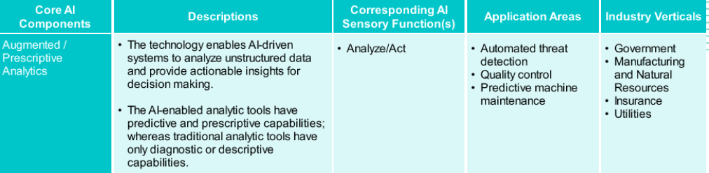
Core AI Components
The following table describes the core components of AI and sample application areas.
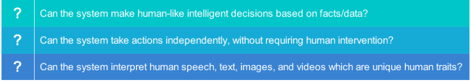
How to identify an AI-Driven System?
If the answer is “yes” to any of these questions, the system uses AI for decision making and taking actions,
What Is Not Al?
A system does not use Al, if it uses:
A set of pre-defined rules to automate human tasks.
ML algorithms to predict something (generated in the form of a report), but there is no action taken based on such predictions.
ML algorithms to find correlations and patterns in the data.
Cognitive technologies to extract information from human speech, text, or videos but there is no action associated with the intelligence derived.
One thumb rule to remember: “If a system is not capable of making independent decisions, it’s not an Al-driven system.”
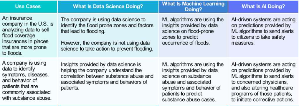
AI Use Cases
Let us look at a few examples of how AI-driven systems are taking actions based on predictions provided by ML algorithms.
Future of AI
More and more organizations are realizing the true value that Al can bring to their organizations. Let us look at some areas where Al can make a big difference.
Al will augment and enhance, rather than automate The ‘Intelligence’ in Al should perceive and behave in human and replace, our human experiences.and familiar ways.
Note of Caution:
“As Al-driven systems make decisions based on ML algorithms, which in turn, rely on data collected from various sources, the systems can sometimes make incorrect, even biased decisions. Therefore it is essential to use diverse data sets and apply ethical standards while developing ML algorithms”.
Applications of AI in real world
Pharma companies can analyze the sales data of the past years to understand the sales pattern of each of its products. Which of the analytics applications can be used? Descriptive analytics! provides an insight into the past and answers the question of what has happened. So, organizations can use descriptive analytics to create a summary of the historical sales data.
Smart email categorization and automatic spam filters used in Gmail is one of the prominent applications of machine learning.
Core Al component can be related to the sensory function- The computer/smart vision component of Al enables systems to extract meaningful and actionable information by analyzing digital images and videos.
A well known real-world application is Chatbots. Using chatbots as virtual personal assistants, the bank can enhance their customer service operations.
Another renowned application is the Al-driven system, the system makes human-like intelligent decisions based on facts/data.
Summary
Al-driven systems can see, talk, listen, analyze or act, and remember information.
The core Al components associated with decision making are:
1. Natural language processing technology.
2. Computer vision technology.
3. Augmented or prescriptive analytics technology.
Before discussing what is an image generator one should be aware of Convolutional Neural Network.
In each image there would be a lot of wasted space, it will be interesting to see if there was a way that we could condense the image down to the important features that distinguish what makes it a shoe, or a handbag, or a shirt. That’s where convolutions come in any kind of image processing, it usually involves having a filter and passing that filter over the image in order to change the underlying image. The process works a little bit like this, for every pixel, take its value, and take a look at the value of its neighbors. The idea here is that some convolutions will change the image in such a way that certain features in the image get emphasized.
Now, that’s a very basic introduction to what convolutions do, and when combined with something called pooling, they can become really powerful. But simply, pooling is a way of compressing an image. A quick and easy way to do this is to go over the image of four pixels at a time i.e., the current pixel and its neighbors underneath and to the right of it. Of these four, pick the biggest value and just keep that. So, for example, my 16 pixels on the left are turned into the four pixels, by looking at them in two-by-two grids and picking the biggest value. This will preserve the features that were highlighted by the convolution, while simultaneously quartering the size of the image. We have horizontal and vertical axes.
We don’t have to do all the maths for filtering and compressing, we will simply define convolutional and pooling layers to do the job for us. So now let’s take a look at convolutions and pooling in code.
model = tf.keras.models.Sequential([
    # Note the input shape is the desired size of the image 150x150 with 3 bytes color
    tf.keras.layers.Conv2D(16, (3,3), activation='relu', input_shape=(150, 150, 3)),
    tf.keras.layers.MaxPooling2D(2,2),
    tf.keras.layers.Conv2D(32, (3,3), activation='relu'),
    tf.keras.layers.MaxPooling2D(2,2),
    tf.keras.layers.Conv2D(64, (3,3), activation='relu'),
    tf.keras.layers.MaxPooling2D(2,2),
    # Flatten the results to feed into a DNN
    tf.keras.layers.Flatten(),
    # 512 neuron hidden layer
    tf.keras.layers.Dense(512, activation='relu'),
    # Only 1 output neuron. It will contain a value from 0-1 where 0 for 1 class ('cats') and 1 for the other ('dogs')
    tf.keras.layers.Dense(1, activation='sigmoid')
])
Every input image is 300×300 pixels, with 3 bytes to define a color(RBG, if it’s the grey image we’ll specify 1 byte). Pooling helps to reduce the information in an image while maintaining features.
Flatten( one of the Neural Network layer) takes input and turns it into a simple linear array.
The interesting stuff happens in the middle layer, sometimes also called a hidden layer.
This model.summary method allows you to inspect the layers of the model, and see the journey of the image through the convolutions, and here is the output.
The model.summary() method call, prints a summary of the Neural Network.
model.summary()
The “output shape” column shows how the size of your feature map evolves in each successive layer. The convolution layers reduce the size of the feature maps by a bit due to padding, and each pooling layer halves the dimensions.
You looked at convolutions and got a glimpse for how they worked. By passing filters over an image to reduce the amount of information, they then allowed the neural network to effectively extract features that can distinguish one class of image from another. You also saw how pooling compresses the information to make it more manageable. This is a really nice way to improve our image recognition performance.
The algorithms we are learning is really the real stuff that is used today in many commercial applications. For example, if you look at the way a real self-driving car today uses cameras to detect other vehicles or pedestrians to try to avoid them, they use convolutional neural networks for that part of the task, very similar to what you are learning. And in fact, in other contexts, using a convolutional neural network for example, we can take a picture of a crop and try to tell if it has a disease coming.
Image Generator in Tensor Flow:
One of the features of the image generator in TensorFlow is that you can point it at a directory and then the sub-directories of that will automatically generate labels for you. So for example, consider this directory structure. You have an image directory and in that, you have sub-directories for training and validation. When you put sub-directories in these for horses and humans and store the requisite images in there, the image generator can create a feeder for those images and auto label them for you. So for example, if I point an image generator at the training directory, the labels will be horses and humans and all of the images in each directory will be loaded and labeled accordingly (Each epoch is loading the data, calculating the convolutions and then trying to match the convolutions to labels.)
Convolutions improve image recognition by isolating the features in images. Applying Convolutions on top of our Deep neural network effects training in many ways it depends on many factors. It might make your training faster or slower, and a poorly designed Convolutional layer may even be less efficient than a plain Deep Neural Network!
Sometimes our training data is close to 1.000 accuracy, but our validation data isn’t, what’s the risk here are probably we were over-fitting on your training data ( this means our model just memorizing the things. Even though our model has 100% training accuracy it cannot predict correctly which it doesn’t train on.) For example, we trained our model to distinguish what is human and what is a horse if it came through some outlier, model will fail to predict the correct one.
Our model may fail to label this one correctly because we too don’t know what to call it as a horse or human or else horseman?
Convolutional Neural Networks are better for classifying images like horses and humans because, In these images, the features may be in different parts of the frame. There’s a wide variety of horses. There’s a wide variety of humans
If we reduce the size of the images, the training results will be different because we removed some convolutions to handle the smaller images. (We need to adjust how many convents i.e., convolutional neural network are needed for the desired accuracy and also we need to adjust neurons accordingly there’s no other way to choose these but some good practices exist.
So, far we have learned how to use TensorFlow to implement a basic neural network, going up all the way to basic Convolutional Neural Network.
So with a smaller data set, you are at great risk of over-fitting; with a larger data set, then you have less risk of over-fitting, but over-fitting can still happen.
We’ll learn another method for dealing with over-fitting, which is that TensorFlow provides very easy to use tools for data augmentation, where you can, for example, take a picture of a cat, and if you take the mirror image of the picture of a cat, it still looks like a cat. So why not do that, and throw that into the training set. Or for example, you might only have upright pictures of cats, but if the cat’s lying down, or it’s on its side, then one of the things you can do is rotate the image. So it’s like part of the image augmentation, rotation, skewing, flipping, moving it around the frame. One of the things I find really fascinating about it is particularly if you’re using a large public data set, is then you flow all the images off directly, and the augmentation happens as it’s flowing. So you’re not editing the images themselves directly. You’re not changing the data set. It all just happens in memory. This is all done as part of TensorFlow’s Image Generation.
So then another strategy, of course for avoiding over-fitting, is to use existing models and to have transfer learning. Yeah. So I don’t think anyone has as much data as they wish, for the problems we really care about. So Transfer Learning, lets you download the neural network, that maybe someone else has trained on a million images, or even more than a million images.
So take an inception network, that someone else has trained, download those parameters, and use that to bootstrap your learning process, maybe with a smaller data set. That has been able to spot features that you may not have been able to spot in your data set, so why not be able to take advantage of that and speed-up training yours. So use transfer learning and TensorFlow lets you do that easily.
Before going to discuss how computer identifies and labels objects let’s understand what is computer vision in detail.
“Computer vision is the field of having a computer understand and label what is present in an image(i.e, this is a dog or cat without being explicitly programmed) and then figure out the patterns.”
You can interpret what a shirt is or what a shoe is, but how would you program for that? if an extra terrestrial who had never seen clothing walked into the room with you, how would you explain the shoes to him? It’s really difficult, if not impossible to do right? And it’s the same problem with computer vision.
So one way to solve that is to use lots of pictures of clothing and tell the computer what that’s a picture of and then have the computer figure out the patterns that give you the difference between a shoe, and a shirt, and a handbag, and a coat.
For example, take a computer vision problem? Let’s take a look at a scenario where we can recognize different items of clothing, trained from a data set containing 10 different types.
Fashion-MNIST is available as a data set with an API call in TensorFlow(Tensorflow has in-built data sets available for learning purposes we just need to import them) but before that let’s start with our import of TensorFlow.
import tensorflow as tf
print(tf.__version__)
The Fashion MNIST data is available directly in the tf.keras datasets API. You load it like below.
mnist = tf.keras.datasets.fashion_mnist
In the MNIST data set, 60,000 of the 70,000 images are used to train the network, and then 10,000 images, one that it hasn’t previously seen, can be used to test just how good or how bad it is performing.
Calling load_data on this object will give you two sets of two lists, these will be the training and testing values for the graphics that contain the clothing items and their labels.
What do these values look like? Let’s print a training image, and a training label to see…Experiment with different indices in the array. For example, also take a look at index 0.
import numpy as np
np.set_printoptions(linewidth=200)
import matplotlib.pyplot as plt
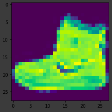
plt.imshow(training_images[0])
print(training_labels[0])
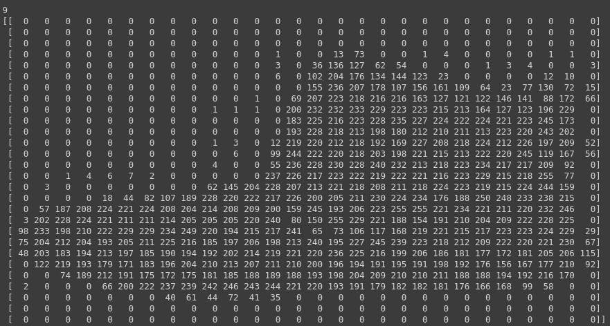
print(training_images[0])
If you notice that all of the values in the number are between 0 and 255. If we are training a neural network, for various reasons it’s easier if we treat all values as between 0 and 1, a process called ‘normalizing‘…and fortunately in Python it’s easy to normalize a list like this without looping.
Now you might be wondering why there are 2 sets…training and testing — remember the idea is to have 1 set of data for training, and then another set of data for testing…that the model hasn’t yet seen…to see how good it would be at classifying values. After all, when you’re done, you’re going to want to try it out with data that it hadn’t previously seen!
Let’s now design the model. There are quite a few new concepts here but don’t worry, you’ll get the hang of them by reading the description below.
model = tf.keras.models.Sequential([tf.keras.layers.Flatten(),
                                    tf.keras.layers.Dense(128, activation=tf.nn.relu),
                                    tf.keras.layers.Dense(10, activation=tf.nn.softmax)])
Sequential: That defines a SEQUENCE of layers in the neural network.
Flatten: Remember earlier where our images were a square when you printed them out? Flatten just takes that square and turns it into a 1-dimensional set.
Dense: Adds a layer of neurons.
Each layer of neurons needs an activation function to tell them what to do. There are lots of options, but just use these for now.
Relu effectively means “If X>0 return X, else return 0” — so what it does it only passes values 0 or greater to the next layer in the network.
Softmax takes a set of values, and effectively picks the biggest one, so, for example, if the output of the last layer looks like [0.1, 0.1, 0.05, 0.1, 9.5, 0.1, 0.05, 0.05, 0.05], it saves you from fishing through it looking for the biggest value, and turns it into [0,0,0,0,1,0,0,0,0] — The goal is to save a lot of coding! as well as time.
The next thing to do, now the model is defined, is to actually build it. You do this by compiling it with an optimizer and loss function as before — and then you train it by calling *model.fit * asking it to fit your training data to your training labels — i.e. have it figure out the relationship between the training data and its actual labels, so in future, if you have data that looks like the training data, then it can make a prediction for what that data would look like.
model.compile(optimizer = tf.optimizers.Adam(),
loss = 'sparse_categorical_crossentropy',
metrics=['accuracy'])
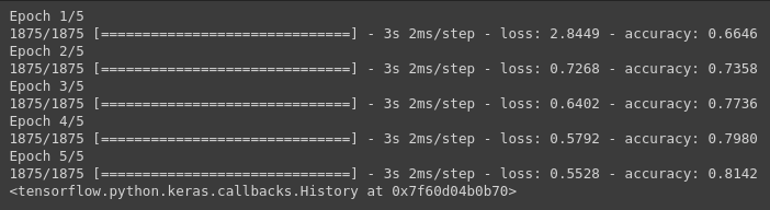
model.fit(training_images, training_labels, epochs=5)
Once it’s done training — you should see an accuracy value at the end of the final epoch. It might look something like 0.8142. This tells you that your neural network is about 81% accurate in classifying the training data. I.E., it figured out a pattern match between the image and the labels that worked 81% of the time. Not great, but not bad considering it was only trained for 5 epochs and done quite quickly.
But how would it work with unseen data? That’s why we have the test images.
We can call the function model.evaluate, and pass in the two sets, and it will report back the loss for each. Let’s take a look.
model.evaluate(test_images, test_labels)
An accuracy that was returned was about .7971, which means it was about 79% accurate. As expected it probably would not do as well with unseen data as it did with data it was trained on! As we move further, there are ways to improve this.
To explore further, let’s create a set of classifications for each of the test images, and then prints the first entry in the classifications.
The output of the model is a list of 10 numbers. These numbers are a probability that the value being classified is the corresponding value, i.e., the first value in the list is the probability that the image is of a ‘0’ (T-shirt/top), the next is a ‘1’ (Trouser), etc. Notice that they are all VERY LOW probabilities.
For the 9 (Ankle boot), the probability was in the ’90s, i.e. the neural network is telling us that it’s almost certainly a 7. The 10th element on the list is the biggest, and the ankle boot is labeled 9. The list has the 10th element being the highest value means that the Neural Network has predicted that the item it is classifying is most likely an ankle boot.
We came to the end, so far we have loaded data, built a model, and fed with training data we predicted ankle boot. A few key points to consider are:
Increase the number of neurons — The impact is training takes longer but results are accurate. By adding more Neurons we have to do more calculations, slowing down the process, but in this case, they have a good impact — we do get more accurate. That doesn’t mean it’s always a case of ‘more is better’, you can hit the law of diminishing returns very quickly!
Remove the Flatten() layer. Why do you think that’s the case you get an error about the shape of the data. It may seem vague right now, but it reinforces the rule of thumb that the first layer in your network should be the same shape as your data. Right now our data is 28×28 images, and 28 layers of 28 neurons would be infeasible, so it makes more sense to ‘flatten’ that 28,28 into a 784×1. Instead of writing all the code to handle that ourselves, we add the Flatten() layer at the beginning, and when the arrays are loaded into the model later, they’ll automatically be flattened for us.
Change final (output) layers — You get an error as soon as it finds an unexpected value. Another rule of thumb — the number of neurons in the last layer should match the number of classes you are classifying for. In this case, it’s the digits 0-9, so there are 10 of them, hence you should have 10 neurons in your final layer.
Consider the effects of additional layers in the network — There isn’t a significant impact — because this is relatively simple data. For far more complex data (including color images to be classified as flowers), extra layers are often necessary.
The impact of training for more or fewer epochs — you might see the loss value stops decreasing, and sometimes increases. This is a side effect of something called ‘over-fitting’ and you need to keep an eye out for when training neural networks. There’s no point in wasting your time training if you aren’t improving your loss, right!
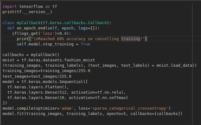
Callbacks — stop the training when I reach the desired value?’ — i.e. 95% accuracy might be enough for you, and if you reach that after 3 epochs, why sit around waiting for it to finish a lot more epochs…So how would you fix that? Like any other program…you have callbacks! Let’s see them in action…
Recommender Systems have taken more and more place in our lives from the last few decades, with the rise of YouTube, Amazon, Netflix and many other such web streaming platform i.e., from e-commerce (suggest to buyers articles that could interest them) to online advertisement (suggest to users the right contents, matching their preferences), recommender systems are today unavoidable in our daily online journeys.
Recommender Systems are really critical in some industries as they can generate a huge revenue and also helps to stand out significantly from competitors. There are many success stories of recommender systems, to mention a few, a few years ago, Netflix organised challenges (the “Netflix prize”) with a prize of 1 million dollars to win, where the goal was to produce a recommender system that performs better than its own algorithm.
In this article, we will go through different paradigms of recommender systems. For each of them, we will present how they work, describe their theoretical basis and metrics to evaluate the performance of recommender system.
What is a Recommender System?
Recommender System captures the pattern of people’s behaviour and use it to predict what else they might want or like.
In a nut shell, recommender systems are algorithms hired to suggest relevant items to users (items being movies to watch, text to read, products to buy or anything else depending on industries).
Applications:-
What to buy.
Where to eat.
Which job to apply to.
Who you should be friends with.
Personalize your experience on the web.
Advantages of Recommender Systems:-
Broader exposure.
Possibility of continual usage or purchase of products.
Provides better experience.
Types:-
There are mainly three types:
i) Content-Based methods.
ii) Collaborative Filtering methods.
Further divided into two types
-> memory-based,
-> model-based
iii) Hybrid methods.
Implementing Recommender Systems:
Memory-based:-
Uses the entire user-item data set to generate a recommendation, uses statistical techniques to users or items.
Develops a model of users in an attempt to learn their preferences.
Models can be created using Regression, Clustering, Classification which are machine learning techniques.
Content-based Filtering:-
It recommends users based on the items they liked and recommends similar items to user that they might like it.
Figures out user’s favourite aspects of an item is, then recommends.
“Show me more of the same of what I have liked before” -> content-based
How it works?
Take a look at user’s data:
input user rating:
A
2
B
10
C
8
user ratings for different movies A, B, C.
Comedy
Adventure
Super hero
Sci-fic
A
0
1
1
0
B
1
1
1
1
C
1
0
1
0
One-hot encoded movies matrix generated from weighing the genres.
Multiply input user ratings and genre matrix to get the user profile.
Comedy
Adventure
Super hero
Sci-fic
A
0
2
2
0
B
10
10
10
10
C
8
0
8
0
Weighted genre matrix.
Comedy
Adventure
Super hero
Sci-fic
18
12
20
10
0.3
0.2
0.33
0.16
Sum up all the individual Genres to get the above table.
With these information we are going to see how to predict for a new movie. Before that see the user profile.
Comedy
Adventure
Super hero
Sci-fic
User
0.3
0.2
0.33
0.16
User profile.
Movies matrix
Comedy
Adventure
Super hero
Sci-fic
1
1
0
1
0
0
1
0
1
0
1
0
The above table is a input user ratings.
Convert the above user input ratings to weighted movies matrix.
0.3
0.2
0
0.16
0
0
0.33
0
0.3
0
0.33
0
Weighted movies matrix.
To get the recommendation matrix take the summation of individual row from the weighted movies matrix. This matrix would assist algorithm to make recommendations to the users by considering weighted average. Like if the average is less it would not recommend if average is high good chances for the item being recommended to the user.
0.66
0.33
0.63
Recommendation matrix.
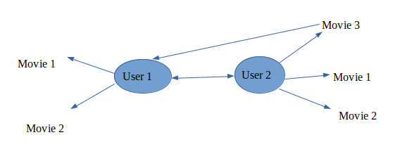
Collaborative Filtering:-
Recommends what is popular among the user neighbour’s and recommends the same item to the user so they might like it.
Makes recommendations based on users of same neighbourhood.
Two types:
i) User-based collaborative filtering: It is based on user’s neighbourhood.
ii) Item-based collaborative filtering: Based on item’s similarity.
Collaborative filtering makes recommendations based on users of same neighbourhood, with whom he/she shares a common preferences and vice-versa for item-based collaborative filtering.
Challenges of Collaborative filtering:
Data Sparsity:- Users in general rate only a limited number of items.
Cold start:- Difficulty in recommendation to new users or new items.
Scalability:- Increase in number of users or items.
TensorFlow is an open-source end-to-end platform for machine learning. It provides a comprehensive ecosystem of tools for developers, enterprises, and researchers who want to push the state-of-the-art of machine learning and build scalable machine learning-powered applications. TensorFlow was designed to help you learn to build models easily. With an intuitive easy-to-use set of APIs that makes it simple for you to learn and implement Machine Learning, Deep Learning and Scientific Computing.
TensorFlow provides a rich collection of tools for building models. These include data pre-processing, data ingestion, model evaluation, visualization and serving.
Data pre-processing the most important step in the data mining process, even though data preparation and filtering process take a significant amount of time. Often, given high value, because to deal with faulty Data-Collection methods resulting in missing values, out-of-range values (e.g., age: 1000). To say a few data pre-processing steps include normalization, transformation, treating missing values etc.,
Data ingestion plays a key role by allowing companies to move, store, integrate and further analyze data across many sources to make predictions and plan for upcoming needs despite many data ingestion challenges includes slow, complex and expensive.
A model evaluation which helps to find out the best model that represents our data as well as how well it will predict. With evaluation metrics, we can measure the goodness of fit between our model and data which emphasises prediction accuracy and to compare different models.
Visualization: TensorBoard is a suite of web applications for examining and understanding model graphs to track and visualize loss and accuracy. TensorBoard supports five visualizations i.e., to display images, text, audio, histograms and graphs.
Serving: TensorFlow serving is designed for production environments. TensorFlow Serving makes it easy to deploy new algorithms.
But it’s not just for building models. You can easily train and deploy your model anywhere with TensorFlow. It’s designed to be highly portable, running on a variety of devices and platforms. It can scale from a single CPU to a GPU or cluster of GPUs, all the way up to a multi-node TPU infrastructure. TensorFlow also allows for powerful experimentation with the flexibility to quickly implement state-of-the-art models, TensorFlow can power your research into new techniques to solve novel problems and solves everyday machine learning problems. From healthcare to social networks and e-commerce, TensorFlow can fit into any industry to solve their biggest problems.
Some case studies
Airbnb improves the guest experience by using TensorFlow to classify images and detect objects at scale.
Carousell uses TensorFlow to improve the buyer and seller experience.
Coca-Cola used TensorFlow to achieve a long-sought frictionless proof-of-purchase capability.
Paypal is using TensorFlow to stay at the cutting edge of Fraud Detection.
Some other use cases include diagnosis of diabetic retinopathy, helping rural farmers spot diseased plants, and predicting extreme weather conditions with fast debugging and the ability to apply state of the art ML models. And to top it all off, TensorFlow derives its roadmap from the needs of its users.
“How machine learning works is that the model will guess the relationship between the numbers”.
Basic Hello World example
Let’s walk through a basic Hello world example of building a machine learning model:
Take a look at these numbers
X = -1, 0, 1, 2, 3, 4,
Y = -3, -1, 1, 3, 5, 7
Can you see the relation between X and Y values?
It is actually Y = 2X – 1.
So, if u see it how did you get that, maybe you noticed Y value increases by 2 and X value increases by only 1. And then you may have seen when X was 0 then Y was -1, we figured Y = 2X – 1. We guessed this and this could work with all the remaining numbers this is the principle all machine leaning works on.
Let’s write a machine learning code that figures out what matches these numbers to each other.
Let’s define the model before writing the simplest possible neural network. A model is a trained neural network which in this case, is a single layer indicated by the ‘keras.layers.Dense code’. What is dense? A dense is a layer of connected neurons.
model = keras.Sequential([keras.layers.Dense(units=1, input_shape=[1])])
This layer has a single neuron in it, indicated by units = 1. We also feed a single value into the neural network which is the X value and we will have the neural network predict what the Y would be for that X. That is why input_shape is one value
model.compile(optimizer = ‘sgd’, loss = ‘mean_squared_error’)
Before compiling model we should know about two functions i.e., the loss and optimizer. These are the key to machine learning. How machine learning works is that the model will guess the relationship between the numbers.
For example, it might guess that Y = 5X + 5. And when training, it will then calculate how good or how bad that guess is, using loss function. And then, it will use the optimizer function to generate another guess. The logic is that the combination of these two functions will slowly get us closer and closer to the correct formula.
In this case, it will go through that loop 500 times, making a guess, calculating how accurate that guess is and then using the optimizer to enhance that guess, and so on. The data itself is set up as an array of Xs and Ys, and our process of matching them to each other is in the fit method of the model. We say, “fit the Xs to the Ys and try this 500 times.”
When it’s done, we will have a trained model. So, now you can try to predict a Y value for a given X.
print(model.predict([10.0]))
Predict the Y when X equals to 10. You might think that the answer is 19, right? But it isn’t. It’s something like 18.9998. It is close to 19, but it’s not quite there. Why do you think that would be?
Well, the computer was trained to match only six pairs of numbers. It looks like a straight-line relationship between them, for those six, but it may not be a straight line for values outside of those six. There’s a very high probability that it is a straight line, but we cannot be certain. And this probability is built into the prediction, so it is telling us very close to 19, instead of exactly 19.
So far, we have learned what is TensorFlow, what tools TensorFlow provides and how to use them and use cases of TensorFlow in real-world which drives impactful solutions to the ultra-modern problems and demonstration of building a basic machine learning model in TensorFlow.