- Können Sie mich hören
- Ich zeige dir
- Wir haben schon besprochen
- Ich gebe weiter an (Person name)
- Kannst du das machen
- Wie weit bist du?
- Wie lange dauert es?
- Ich habe heute einen Termin mit (Person name)
- Ich gebe dir Bescheid.
- Ich schreibe dir
- Wenn du Hilfe brauchst, kannst du dich gerne an mich wenden.
- Wenn du fragen hast, kannst du mir gerne schreiben.
- Falls du Hilfe brauchst, kannst du dich gerne jederzeit an mich wenden.
- Bei Rückfragen, stehe ich gerne zur Verfügung.
- Wir haben das schon ausgemacht.
- Wir müssen einen Termin setzen.
- Ich habe gestern mit der Klasse 1 gearbeitet.
- Ich werde heute mit diesem Thema beschäftigen
- Ich verabschiede mich.
- Was machst du
- Was hast du heute gemacht
- Ich teile gleich meinen Bildschirm
- Kannst du bitte deinen Bildschirm teilen.
- Ich höre Sie nicht.
- Ich könnte nicht hören
- Wie kann ich dir helfen
- Ich bin dabei
- Ich kann das übernehmen
- Ich setze einen Termin.
- Ich werde heute mit (Person Name) abstimmen.
- Ich stimme mit (Person Name) ab.
- Es geht weiter um viertel vor eins.
- Ich mache jetzt eine kurze Pause.
- Du bist herzlich eingeladen.
- Ich melde mich später
- Meldest du dich bitte bei (Person Name)
- Wie lauft bei dir?
- Hast du etwas zu schreiben?
- Kannst du bitte enter drücken
- Kannst du bitte das Dialog Fenster zumachen
- Klicken Sie auf ‚OK‘ Schaltfläche
- Geben Sie bitte Ihre Benutzername und Kennwort ein.
- Hast du das verstanden?
- Ich habe das verstanden
- Kommst du einige maßen zurecht?
- Wir freuen uns, Ich freue mich.
- Kannst du mir eine E-Mail schreiben?
- Ich habe eine E-Mail an dich geschickt.
- Bitte um überprüfen
- Sieht Ihr meinen Bildschirm.
- Kannst du mich in zehn Minuten anrufen?
- Ich rufe in 10 Minuten an
- Um 15 Uhr passt bei dir? Das passt bei mir
- Das stimmt
- Du hast Recht
- Wie sieht aus bei dir
- Ich habe Sie/dich gerade telefonisch leider nicht erreicht.
Author: Raja Rajeswari Kannan
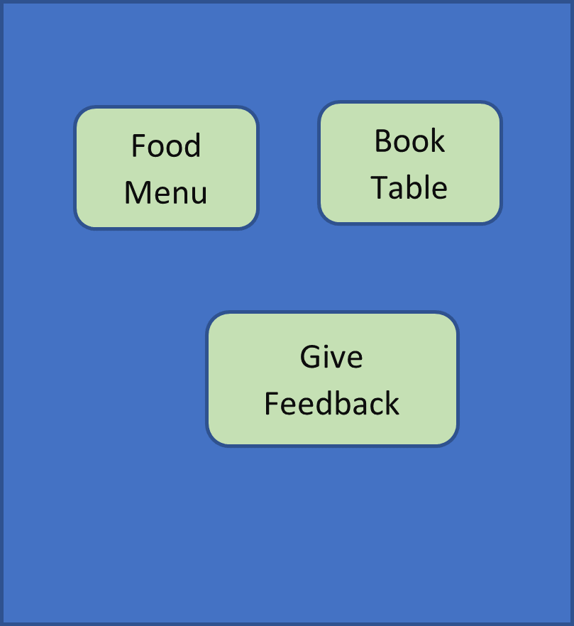
How to serve food without any contact in Restaurant using Corona App
Objective:
The main purpose of the App is to provide food services at the restaurant with minimum contact. It also includes managing the customer service tables to ensure appropriate distance between two customers. The Food Service is digitalised with the menu options available through the App. The information of the customer is stored based on the customer preference. The customer feedbacks are analysed to improve the food service. The complete restaurant services can be administered centrally using the App.
Major features of the App:
- The Food service tables are digitalised.
- The Food menu options are controlled dynamically through the App.
- The data flow between the service tables and the kitchen service can be controlled through the App.
- The customer feedbacks and the sales are analysed using Lean Management Techniques.
- The critical customer information can be managed centrally with a client no with the consent of the customer.
- The pre-order options can be available based on the Restaurant needs.
Food Service Table:
The QR Bar code option can be used to uniquely identify the food service table. customer cannot enter any random no to book the Food Service Table.
Menu Options:
The menu options should always be dynamic displayed on the current day options. In case if a food item is not available during a day, then it should automatically be hidden from the display. The special menu for the day can be highlighted.
Kitchen Service:
The Kitchen Service is alerted centrally using a Display that is controlled by the main service pattern. The data flow between the customer and kitchen Service must be fast and transparent.
Customer Feedbacks:
The customer orders and feedbacks are analysed daily, weekly, monthly. Lean principles must highlight the food with high revenue. It should also indicate peak service time during each day. The app must help in solving the customer feedbacks, on the next subsequent corresponding customer visit. The respective customer and the restaurant manger must be aware of the resolved issue.
Pre-order Option:
The App gives an option to book the food service table in advance.
Critical points for the development of the App:
- The customer data can be stored as a client no in the server centrally. The actual customer data must always be stored locally with restaurant manager. This ensure that the customer data is protected to the maximum.
- The App, storage cost is estimated against the return on investment.
- The data flow between the different point, must be checked with parameters such as data size.
- The Food Menu options must always be dynamically controlled with less inputs from the App user (Restaurant manager).
- Secure payment options can be an additional feature.
Market Analysis:
The App is specifically suited for the local German markets for the following reasons:
- Customer data being stored locally with the restaurant.
- Current pandemic situation enforces less contact in public places such as restaurants. German locals wish to enjoy the Restaurant atmosphere rather than placing the order from home.
- Simple to develop features such as QR barcode and local storage implementation
- One real time case is Vapiano restaurant which had to close due to the loss incurred during the pandemic.
| Parameters | Current proposal |
| Book orders | |
| Customer reviews | |
| Payment service | |
| Local table control option | |
| Local data storage |
| Tasks |
| User Interface, Database Architecture |
| Object model, Framework, Business logic |
| Testing |
| Implementation |
User Interface:

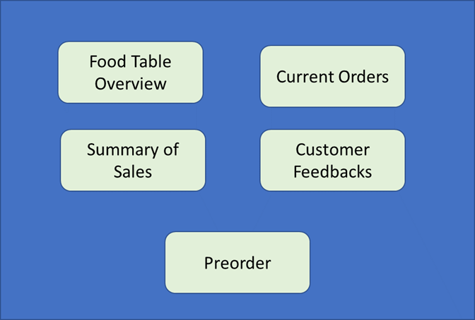
Restaurant Manager


Conclusion:
The App solves the current pandemic issue with less contact in the Restaurant. The Restaurant can be controlled centrally, and its sales can be monitored every hour. It is an affordable App to meet the local requirements of a restaurant and all the data are stored to only a confined network.
How Data and Analytics Are Driving Digital Business?
In this article, we will discuss how data and analytics are impacting business and in our day-to-day lives and how important in digital businesses and their applications in the real world.
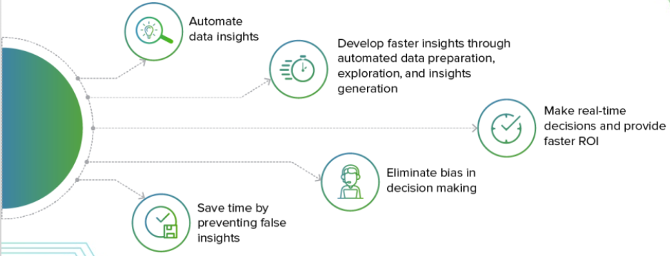
In the past, organizations would use analytic applications mainly for enterprise data reporting. However, more and more organizations are now using data and analytics as raw materials for enterprise-level decision making. The following flowcharts illustrate this point:


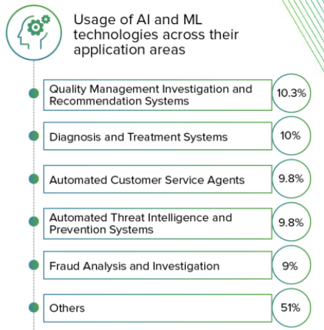
The Current Al Wave Is Poised to Finally Break Through.
Al is becoming fast a core business and analytical competency. Al and ML technologies are providing rapidly improved decision making and process optimization capabilities to organizations.
By doing so, these technologies promise to:
- Transform business processes.
- Reconfigure workforces.
- Optimize infrastructure behavior.
- Blend industries.

Natural Language Technologies Become Mainstream.
One of the key aspects of Al-driven systems is their ability to process natural language, which is human
speech and text. Natural language is beginning to play a dual role in many organizations.
Examples of Natural Language Processing (NLP):
- Machine Translation: Google translate services.
- Customer Service: NLP is being used in customer service contact centers to understand customer intent, pain-points, and to provide enhanced customer satisfaction.
Examples of Natural Language Generation:
- Generating automated product descriptions from inventory data.
- Creating individual financial portfolio summaries and updates at scale.
- Business intelligence performance dashboard text explanations
- Automated personalized customer communications.
Augmented analytics draws on ML, AI, and natural language generation technologies to:

Applications in real world:
The combination of emerging technologies such as AI, ML, and cloud are often marketed using the following:
• Cognitive Cloud
• Al as a Service
• Intelligent Cloud
A major telecom company wants to enhance its contact center operations by understanding its customers better through their customer care calls, feedback survey responses, and social media interactions. Which Al and analytics application
areas will be useful? In the given scenario, speech recognition and Natural Language processing will help the business enhance its contact center operations.
Google Maps analyzes the speed of traffic through anonymous data locations from smartphones. This enables Google to suggest the fastest routes. Which technology enables Google to do this? AI and ML! Smart machines and applications are steadily becoming a daily Cloud Computing phenomenon, helping us make faster and accurate decisions.
Google Maps uses Al and ML to analyze the speed of traffic Al and ML and suggest the fastest routes.
The Winning Strategy.
What will it take to win in the new digital era? Winning strategy for future growth addressed by the following key business drivers:
Reset the rules of business.
Strategy and Innovation:
- Accelerate innovation.
- Redefine industry operating models.
- Drive growth while reducing risk.
- Enable Change adoption.
Focus on human needs.
Interactive Experiences:
- Combine the best of human science, design thinking, user experience, and technology to provide new end-to-end services for marketers.
- Deliver on the promise of social and brand.
- Build Omnichannel success.
Make intelligent choices.
AI & Analytics:
- Build intelligence-based businesses.
- Make data an asset, not a liability.
- Apply Analytics and Al platforms to fuel growth.
Enable the internet of things.
Connected Products:
- Instrument and connect everything.
- Rapid prototyping and product development.
- Grow revenue from data-driven services.
Build software for the digital economy.
Software Engineering:
- Embed human-insight and design into engineering.
- New tech for new value: Cloud Foundry stack services, micro-services, APIs, engaging interfaces, etc.
- Application portfolio optimization.
This is how organisations leverage its Al and analytics capability to help its clients stay ahead of the competition.
Industry Aligned Solutions.
Every organization will have pre-built solutions to address the needs of the vertical markets. For example,
Google’s Product Data Management solution, which uses Product Intelligence as a service offering,
caters to the needs of the Consumer Goods and Retail verticals. These pre-built solutions are easy to
customize and can be deployed quickly.
Some of the vertical markets:
- Banking.
- Insurance.
- Life Sciences.
- Healthcare.
- Manufacturing & Logistics.
- Comm & IME & Tech.
- Energy & Utilities.
- Consumer Goods & Retail.
- Travel & Hospitality.
Case Study: Opioid addiction and early detection of drug-seeking behavior.
Challenge:
A healthcare firm approached Google for a solution to reduce the number of deaths due to drug misuse.
Solution:
Google developed an Al solution that could seamlessly scan through a physician’s prescription notes and mine for indicators of drug-seeking behavior.
Outcome:
Google’s solution helped the healthcare firm save more than $60M by identifying around 85000 drug seekers before they turned into addicts.
Summary
So far, we have discussed six strategic offerings include:
- Insight to Al.
- Adaptive Data Foundation.
- Risk and Fraud Intelligence.
- Customer 360-degree Intelligence.
- Business Operations Intelligence.
- Product Intelligence.
- Organizations will have pre-built solutions to address the needs of vertical markets.
What Is AI? and What is not AI?
In this article. we’ll discuss AI in detail, and talk about Components of AI and Use Cases, applications of AI in real-world.
Al refers to the ability of machines to perceive, learn, interact with the environment, analyze, and solve problems independently.
Let us take a closer look at how Al-driven systems interact with our environment. Like us humans, Al-driven systems can see, listen, talk, remember information, and analyze/act.
We refer to these capabilities of Al-driven systems as five Al senses, and the technologies associated with these senses are known as core Al components.
The core components are the central building blocks of Al-driven systems, based on which user applications are developed.
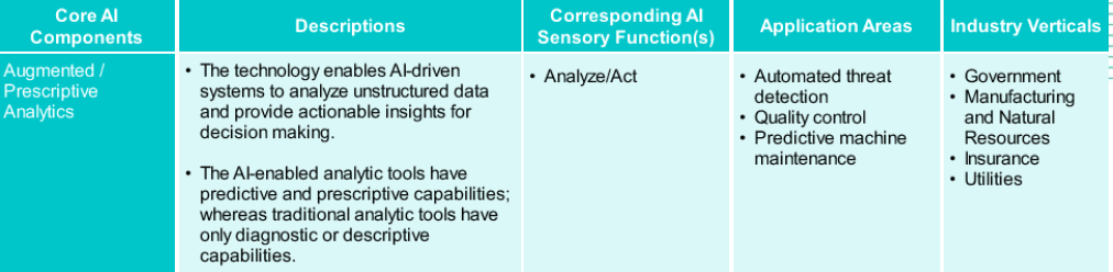
Core AI Components
The following table describes the core components of AI and sample application areas.


How to identify an AI-Driven System?

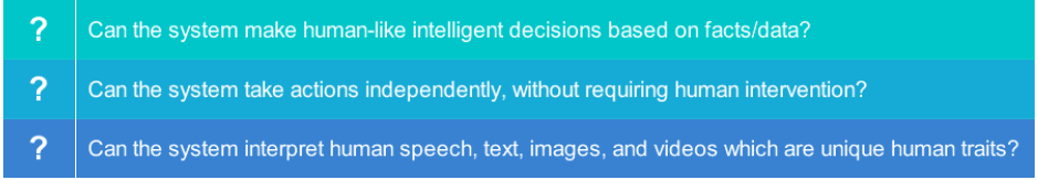
What Is Not Al?
A system does not use Al, if it uses:
- A set of pre-defined rules to automate human tasks.
- ML algorithms to predict something (generated in the form of a report), but there is no action taken based on such predictions.
- ML algorithms to find correlations and patterns in the data.
- Cognitive technologies to extract information from human speech, text, or videos but there is no action associated with the intelligence derived.
One thumb rule to remember: “If a system is not capable of making independent decisions, it’s not an Al-driven system.”
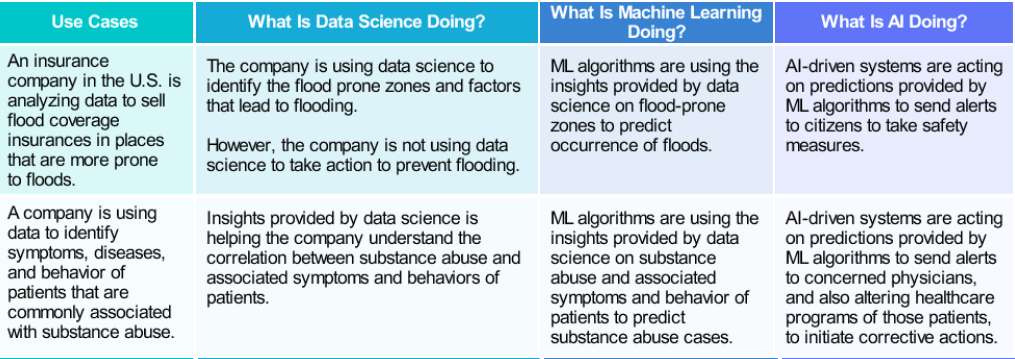
AI Use Cases
Let us look at a few examples of how AI-driven systems are taking actions based on predictions provided by ML algorithms.

Future of AI
More and more organizations are realizing the true value that Al can bring to their organizations. Let us
look at some areas where Al can make a big difference.


and replace, our human experiences. and familiar ways.
Note of Caution:
“As Al-driven systems make decisions based on ML algorithms, which in turn, rely on data collected from various sources, the systems can sometimes make incorrect, even biased decisions. Therefore it is essential to use diverse data sets and apply ethical standards while developing ML algorithms”.
Applications of AI in real world
- Pharma companies can analyze the sales data of the past years to understand the sales pattern of each of its products. Which of the analytics applications can be used? Descriptive analytics! provides an insight into the past and answers the question of what has happened. So, organizations can use descriptive analytics to create a summary of the historical sales data.
- Smart email categorization and automatic spam filters used in Gmail is one of the prominent applications of machine learning.
- Core Al component can be related to the sensory function- The computer/smart vision component of Al enables systems to extract meaningful and actionable information by analyzing digital images and videos.
- A well known real-world application is Chatbots. Using chatbots as virtual personal assistants, the bank can enhance their customer service operations.
- Another renowned application is the Al-driven system, the system makes human-like intelligent decisions based on facts/data.
Summary
- Al-driven systems can see, talk, listen, analyze or act, and remember information.
- The core Al components associated with decision making are:
- 1. Natural language processing technology.
- 2. Computer vision technology.
- 3. Augmented or prescriptive analytics technology.
- 4. Smart data discovery technology
Overview of Analytics- Industry Level!
In this article, we will discourse on organizational level Analytics, Data Science, and its use cases in the corporate world, Machine Learning and its types and use cases, Deep Learning and how does it work.
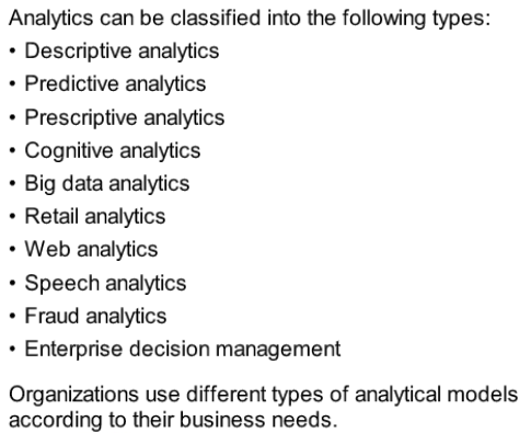
What is Analytics
Analytics is the study of data, collected from various sources, to gain insights into a problem.
Types of Analytics

What is Data Science?
Data science uses a mix of tools, robust programming instructions, and principles of machine
learning to process large amounts of unstructured and semi-structured data, to:
- Identify Patterns from the Collected Data Sets.
- Identify the Occurrence of a Particular Event in the Future.


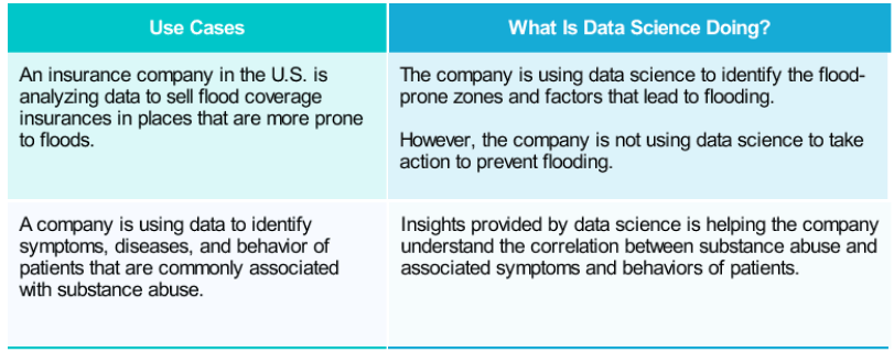
Data Science Use Cases.
Let us look at a few examples of how data science is providing valuable insights to organizations.

What Is Machine Learning?

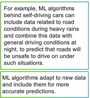
Machine learning (ML) takes off from where data science ends. While data science relies completely
on programming instructions to detect patterns, ML is adaptive in nature. It gives computer systems
the ability to learn and make predictions by processing data and experiences.
Types of Analytics Used by Machine Learning
ML mainly uses predictive analytics.
Given here are a few key features of predictive analytics.


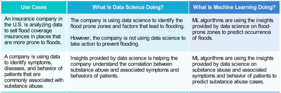
Machine Learning Use Cases
Let us look at a few examples of how ML algorithms are using insights provided by data science to
make predictions.
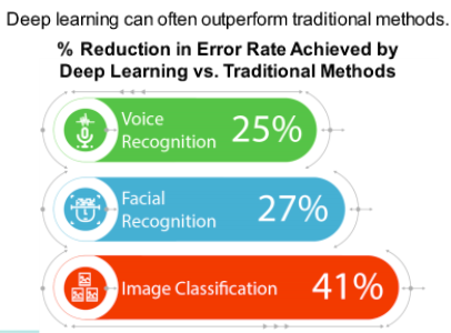
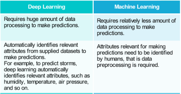
What Is Deep Learning?
Deep learning is an advanced form of ML. It processes a huge amount of data, collected from a wider
range of data sources, and requires very fewer data preprocessing by humans.


How Does Deep Learning Work?
Deep learning uses interconnected layers of software-based calculators, known as “neurons.”
Together, the “neurons” form a neural network, which can ingest a vast amount of data and processes
them through multiple layers. Each layer learns something about the complex features of the data.
Finally, the network makes a determination about that data, assesses whether the determination is correct,
and applies what it has learned to make determinations about new data.


For example, once a neural network learns what an object looks like, it can identify that object in a new image.
In this article, you have learned that:
- Analytics is the study of data, collected from various sources, to gain insights into a problem.
- Data Science gives organizations insights into business problems by processing semi-structured and unstructured data.
- ML algorithms use insights provided by data science to make predictions about future events.
Cats Vs Dogs: A kaggle Challange.
So far we have learned how to use TensorFlow to implement a basic neural network, going up all the way to a basic Convolutional Neural Network. In this article, we’ll go much further by taking the ideas we’ve learned and applied them to a much bigger dataset of cats versus dogs on Kaggle. Yes, so we take the full Kaggle dataset of 25,000 cats versus dogs images. So we want to take a look at what it’s like to train a much larger data set, and that was like a data science challenge, not that long ago. Now, we’re going to learn that here, which I think is really helpful to get great results while operating on much bigger data sets.
What does it take to download a public dataset of the Internet, like cats versus dogs, and get a neural network to work on it? Data is messy, sometimes you find astonishing things like pictures of people holding cats or multiple cats or surprising things in data. For example, you might have some files that are zero length and they could be corrupt as a result. So it’s like using your Python skills, using your TensorFlow skills to be able to filter them out. Building a convolutional neural network to be able to spot things like we mentioned, a person holding a cat. So that’s some of the things we need to concentrate on. We’ll be using a very clean dataset that we’re using with cats versus dogs, but you’re going to hit some of those issues. In this article, you’ll learn the skills that you need to be able to deal with other datasets that may not be as clean as this one.
The reality is, there’s a lot of data cleaning, and having great tools to help with that data cleaning makes our workflow much more efficient. Definitely, in this article, you will get to practice all that, as well as train a pretty cool neural network to classify cats versus dogs. Please go ahead.
In this article, we’ll take our understanding of the Convolutional Neural Network to the next level by recognizing sophisticated real images of Cats and Dogs in order to classify an incoming image as one or the other. In particular, the handwriting recognition made your life a little easier by having all the images be the same size and shape, and they were all monochrome color. Real-world images aren’t like that — they’re in different shapes, aspect ratios, etc, and they’re usually in color!
So, as part of the task you need to process your data — not least resizing it to be uniform in shape.
You’ll follow these steps:
- Explore the Example Data of Cats and Dogs.
- Build and train a Neural Network to recognize the difference between the two.
- Evaluate Training and Validation accuracy.
Explore the Example Data
Let’s start by downloading our example data, a .zip of 2,000 JPG pictures of cats and dogs, and extracting it locally in /tmp.
NOTE: The 2,000 images used in this exercise are excerpted from the “Dogs vs. Cats” dataset available on Kaggle, which contains 25,000 images. Here, we use a subset of the full dataset to decrease training time.
!wget --no-check-certificate \
  https://storage.googleapis.com/mledu-datasets/cats_and_dogs_filtered.zip \
  -O /tmp/cats_and_dogs_filtered.zip
The following python code will use the OS library to use Operating System libraries, giving you access to the file system, and the zip file library allowing you to unzip the data.
import os
import zipfile

local_zip = '/tmp/cats_and_dogs_filtered.zip'

zip_ref = zipfile.ZipFile(local_zip, 'r')

zip_ref.extractall('/tmp')
zip_ref.close()
The contents of the .zip are extracted to the base directory /tmp/cats_and_dogs_filtered, which contains train and validation subdirectories for the training and validation datasets, which in turn each contain cats and dogs subdirectories.
In short: The training set is the data that is used to tell the neural network model that ‘this is what a cat looks like’, ‘this is what a dog looks like’ etc. The validation data set is images of cats and dogs that the neural network will not see as part of the training, so you can test how well or how badly it does in evaluating if an image contains a cat or a dog.
One thing to pay attention to in this sample: We do not explicitly label the images as cats or dogs. If you remember with the handwriting example earlier, we had labeled ‘this is a 1’, ‘this is a 7’ etc. Later you’ll see something called an ImageGenerator being used — and this is coded to read images from subdirectories, and automatically label them from the name of that subdirectory. So, for example, you will have a ‘training’ directory containing a ‘cats’ directory and a ‘dogs’ one. ImageGenerator will label the images appropriately for you, reducing a coding step.
Let’s define each of these directories:
base_dir = '/tmp/cats_and_dogs_filtered'

train_dir = os.path.join(base_dir, 'train')
validation_dir = os.path.join(base_dir, 'validation')

# Directory with our training cat/dog pictures
train_cats_dir = os.path.join(train_dir, 'cats')
train_dogs_dir = os.path.join(train_dir, 'dogs')

# Directory with our validation cat/dog pictures
validation_cats_dir = os.path.join(validation_dir, 'cats')
validation_dogs_dir = os.path.join(validation_dir, 'dogs')
We can find out the total number of cat and dog images in the train and validation directories:
print('total training cat images :', len(os.listdir(train_cats_dir)))
print('total training dog images :', len(os.listdir(train_dogs_dir)))

print('total validation cat images :', len(os.listdir(validation_cats_dir)))
print('total validation dog images :', len(os.listdir(validation_dogs_dir)))
For both cats and dogs, we have 1,000 training images and 500 validation images.
Now let’s take a look at a few pictures to get a better sense of what the cat and dog datasets look like. First, configure the matplot parameters:
%matplotlib inline

import matplotlib.image as mpimg
import matplotlib.pyplot as plt

# Parameters for our graph; we'll output images in a 4x4 configuration
nrows = 4
ncols = 4

pic_index = 0 # Index for iterating over images
Now, display a batch of 8 cat and 8 dog pictures. You can rerun the cell to see a fresh batch each time:
# Set up matplotlib fig, and size it to fit 4x4 pics
fig = plt.gcf()
fig.set_size_inches(ncols*4, nrows*4)

pic_index+=8

next_cat_pix = [os.path.join(train_cats_dir, fname)
                for fname in train_cat_fnames[ pic_index-8:pic_index]
               ]

next_dog_pix = [os.path.join(train_dogs_dir, fname)
                for fname in train_dog_fnames[ pic_index-8:pic_index]
               ]

for i, img_path in enumerate(next_cat_pix+next_dog_pix):
  # Set up subplot; subplot indices start at 1
  sp = plt.subplot(nrows, ncols, i + 1)
  sp.axis('Off') # Don't show axes (or gridlines)

  img = mpimg.imread(img_path)
  plt.imshow(img)

plt.show()
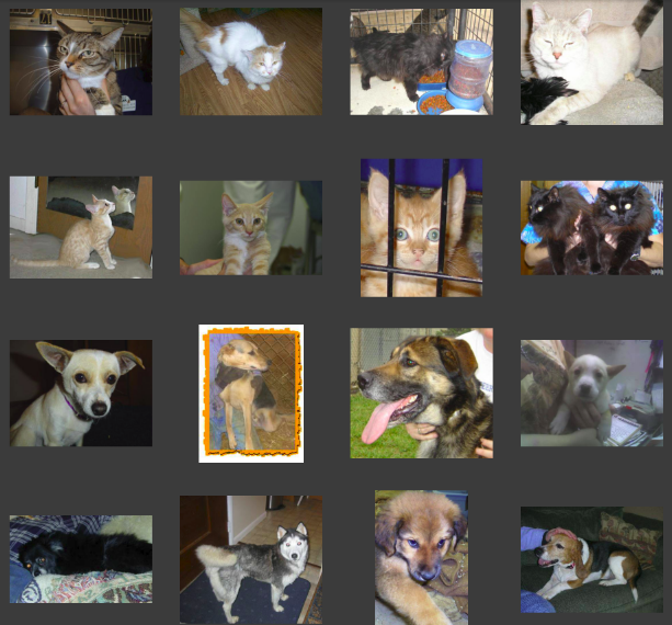
It may not be obvious from looking at the images in this grid, but important note here, and a significant difference is that these images come in all shapes and sizes. These are color and in a variety of shapes. Before training a Neural network with them you’ll need to tweak the images. You’ll see that in the next section.
Ok, now that you have an idea of what your data looks like, the next step is to define the model that will be trained to recognize cats or dogs from these images
Building a Small Model from Scratch to Get to ~72% Accuracy
In the previous section, you saw that the images were in a variety of shapes and sizes. In order to train a neural network to handle them, you’ll need them to be in a uniform size. We’ve chosen 150×150 for this, and you’ll see the code that preprocesses the images to that shape shortly.
But before we continue, let’s start defining the model:
Step 1 will be to import tensorflow
Next, we will define a Sequential layer as before, adding some convolutional layers first. Note the input shape parameter this time. In the earlier example, it was 28x28x1, because the image was 28×28 in greyscale (8 bits, 1 byte for color depth). This time it is 150×150 for the size and 3 (24 bits, 3 bytes) for the color depth.
We then add a couple of convolutional layers as in the previous example and flatten the final result to feed into the densely connected layers.
Finally we add the densely connected layers.
Note that because we are facing a two-class classification problem, i.e. a binary classification problem, we will end our network with a sigmoid activation, so that the output of our network will be a single scalar between 0 and 1, encoding the probability that the current image is class 1 (as opposed to class 0).
model = tf.keras.models.Sequential([
    # Note the input shape is the desired size of the image 150x150 with 3 bytes color
    tf.keras.layers.Conv2D(16, (3,3), activation='relu', input_shape=(150, 150, 3)),
    tf.keras.layers.MaxPooling2D(2,2),
    tf.keras.layers.Conv2D(32, (3,3), activation='relu'),
    tf.keras.layers.MaxPooling2D(2,2),
    tf.keras.layers.Conv2D(64, (3,3), activation='relu'),
    tf.keras.layers.MaxPooling2D(2,2),
    # Flatten the results to feed into a DNN
    tf.keras.layers.Flatten(),
    # 512 neuron hidden layer
    tf.keras.layers.Dense(512, activation='relu'),
    # Only 1 output neuron. It will contain a value from 0-1 where 0 for 1 class ('cats') and 1 for the other ('dogs')
    tf.keras.layers.Dense(1, activation='sigmoid')
])
The model.summary() method call prints a summary of the NN
model.summary()
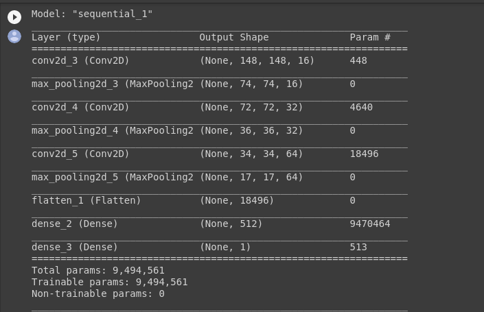
The “output shape” column shows how the size of your feature map evolves in each successive layer. The convolution layers reduce the size of the feature maps by a bit due to padding, and each pooling layer halves the dimensions.
Next, we’ll configure the specifications for model training. We will train our model with the loss because it’s a binary classification problem and our final activation is a sigmoid. We will use the rmsprop optimizer with a learning rate of 0.001. During training, we will want to monitor classification accuracy.
NOTE: In this case, using the RMSprop optimization algorithm is preferable to stochastic gradient descent (SGD), because RMSprop automates learning-rate tuning for us. (Other optimizers, such as Adam and Adagrad, also automatically adapt the learning rate during training, and would work equally well here.)
from tensorflow.keras.optimizers import RMSprop

model.compile(optimizer=RMSprop(lr=0.001),
              loss='binary_crossentropy',
              metrics = ['accuracy'])
Data Preprocessing
Let’s set up data generators that will read pictures in our source folders, convert them to tensors, and feed them (with their labels) to our network. We’ll have one generator for the training images and one for the validation images. Our generators will yield batches of 20 images of size 150×150 and their labels (binary).
As you may already know, data that goes into neural networks should usually be normalized in some way to make it more amenable to processing by the network. (It is uncommon to feed raw pixels into a convent.) In our case, we will preprocess our images by normalizing the pixel values to be in the [0, 1] range (originally all values are in the [0, 255] range).
In Keras, this can be done via the keras.preprocessing.image.ImageDataGenerator class using the rescale parameter. This ImageDataGenerator the class allows you to instantiate generators of augmented image batches (and their labels) via .flow(data, labels) or .flow_from_directory(directory). These generators can then be used with the Keras model methods that accept data generators as inputs: fit, evaluate_generator, and predict_generator.
from tensorflow.keras.preprocessing.image import ImageDataGenerator

# All images will be rescaled by 1./255.
train_datagen = ImageDataGenerator( rescale = 1.0/255. )
test_datagen  = ImageDataGenerator( rescale = 1.0/255. )

# --------------------
# Flow training images in batches of 20 using train_datagen generator
# --------------------
train_generator = train_datagen.flow_from_directory(train_dir,
                                                    batch_size=20,
                                                    class_mode='binary',
                                                    target_size=(150, 150))
# --------------------
# Flow validation images in batches of 20 using test_datagen generator
# --------------------
validation_generator =  test_datagen.flow_from_directory(validation_dir,
                                                         batch_size=20,
                                                         class_mode  = 'binary',
                                                         target_size = (150, 150))
Training
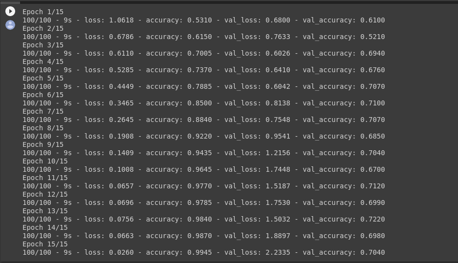
Let’s train on all 2,000 images available, for 15 epochs, and validate on all 1,000 test images.
Do note the values per epoch.
You’ll see 4 values per epoch — Loss, Accuracy, Validation Loss and Validation Accuracy.
Loss and Accuracy are a great indication of the progress of training. It’s making a guess as to the classification of the training data, and then measuring it against the known label, calculating the result. Accuracy is the portion of correct guesses. The Validation accuracy is the measurement with the data that has not been used in training. As expected this would be a bit lower. You’ll learn about why this occurs in the section on overfitting later in this course.
history = model.fit(train_generator,
                              validation_data=validation_generator,
                              steps_per_epoch=100,
                              epochs=15,
                              validation_steps=50,
                              verbose=2)
Evaluating Accuracy and Loss for the Model
Let’s plot the training/validation accuracy and loss as collected during training:
#-----------------------------------------------------------
# Retrieve a list of list results on training and test data
# sets for each training epoch
#-----------------------------------------------------------
acc      = history.history[     'accuracy' ]
val_acc  = history.history[ 'val_accuracy' ]
loss     = history.history[    'loss' ]
val_loss = history.history['val_loss' ]

epochs   = range(len(acc)) # Get number of epochs

#------------------------------------------------
# Plot training and validation accuracy per epoch
#------------------------------------------------
plt.plot  ( epochs,     acc )
plt.plot  ( epochs, val_acc )
plt.title ('Training and validation accuracy')
plt.figure()

#------------------------------------------------
# Plot training and validation loss per epoch
#------------------------------------------------
plt.plot  ( epochs,     loss )
plt.plot  ( epochs, val_loss )
plt.title ('Training and validation loss'   )
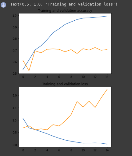
As you can see, we are overfitting like it’s getting out of fashion. Our training accuracy (in blue) gets close to 100% (!) while our validation accuracy (in green) stalls as 70%. Our validation loss reaches its minimum after only five epochs.
Since we have a relatively small number of training examples (2000), overfitting should be our number one concern. Overfitting happens when a model exposed to too few examples learns patterns that do not generalize to new data, i.e. when the model starts using irrelevant features for making predictions. For instance, if you, as a human, only see three images of people who are lumberjacks, and three images of people who are sailors, and among them, the only person wearing a cap is a lumberjack, you might start thinking that wearing a cap is a sign of being a lumberjack as opposed to a sailor. You would then make a pretty lousy lumberjack/sailor classifier.
Overfitting is the central problem in machine learning: given that we are fitting the parameters of our model to a given dataset, how can we make sure that the representations learned by the model will be applied to data never seen before? How do we avoid learning things that are specific to the training data?
In the next exercise, we’ll look at ways to prevent overfitting in the cat vs. dog classification model.
SAP HANA
- The data is handled through in-memory technology in the working space
- The Tables are stored in a column-based manner
- The secondary indexes are not needed anymore
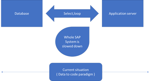
- The new database is based on code-to-data paradigm
- Value compression

- In-memory technology
Neue ABAP-Function for Code-to-data paradigm.
- CASE Statement
- UNION Funktion
- CDS Views on the application server
- SAP List viewer with integrated data access (showing the data directly from the database)


The Server today is costly due to the performance issues and large memory space is needed for the RAM.
SAP HANA is used to save the memory space by bringing in-memory technology.
Persistence view is used to hold the data in following cases.
- When the data occupies more space in the hard disk.
- When the server is down
- The changes in the data records will be saved in the logs. Those changes will be updated on the HANA database and the buffer will be deleted.
- The changes in the column-based data tables cannot be saved directly. The data has to be organised with the help of temporary tables, before it is saved to the column based tables.
2. SAP HANA Column based approach:
Example Data table:
| Food item | Food Id | Food cost | Currency |
| Cool drink | 100 | 20 | INR |
| Cheese burger | 101 | 30 | INR |
| Ice cream | 102 | 15 | INR |
- Column based approach:
Both row based and column based approaches are possible in SAP HANA .
Column based approach: This approach is useful for aggregation purpose. For example in order to find the total cost of the food items, the column based approach is useful as the total can be determined in a single line.
- Row based approach:
This approach is useful for transactional data. For example in order to change the currency of a particular food item.
In the column based approach, when we insert a single line ( One column ), the table needs to be reorganised before it is saved.
The column based and rows based selection options are available from SAP Netweaver ABAP 7.4 version through ABAP Dictionary (SE11 Transaction).
3. Value compression
In the column-based approach, there is only one data type for a series of values in the column. It makes it easy to compress via attribute vector.
A compressed column will be created with every value and a numerical id is assigned to it. An inverted index table is created with the index ids and lines.
| Inverted Table | |
| Index | lines |
Working with numbers is easier than strings. String operations takes a lot of load on the central processing unit.
A Practical approach to Enterprise Resource Planning
In this post, we will explain the ERP concept with Retail store as an example. Questions such as how retail store functions and how retail store functions are related to ERP are answered.
Let us consider initially important components in a Retail operation. The components such as Warehouse, Storage location, Shoe retail store, Billing and procurement of shoes play a crucial role in Retail operation.
We will consider shoe sales in a retail store.
The shoes are sold in various locations such as chennai, Bangalore, Delhi. These retails stores can be uniquely identified using shop_no_001 etc. The shoes in the retail store are stocked initially in a warehouse center. This warehouse center can be within the shop or at a remote location. Within each warehouse centers, there are different storage locations, in order to store shoes of different types and brands.
Lets now move to the other side of the retail operation. The shoes can be purchased by two set of purchasing groups such as office employees and college youth. we can classify these groups as formal and informal shoes.
The shoe sales is figured out using the POS (point of sales) system.
The following table of data are critical in such an ERP system.
| Shoe data | |
| Material | Shoes Bata |
| Material number | SHOES_BATA |
| total shoes | 200 |
| unit of measure | Pieces |
| Available from | 1st January 2020 |
| Net weight | 10 kg |
| processing time | 1 hour |
| Shoe shop list | ||
| material | shoe shop store | shoe store location |
| SHOES_BATA | 001 | Chennai |
| SHOES_BATA | 002 | Bangalore |
| SHOES_BATA | 003 | Delhi |
| Warehouses for shoes | ||
| material | shoe store | warehouse number |
| SHOES_BATA | 002 | WAREHOUSE_NO_001 |
| SHOES_BATA | 002 | WAREHOUSE_NO_002 |
| Storage locations for shoes in Warehouse no 001 in bangalore location | |||
| material | shoe store | warehouse number | storage location |
| SHOES_BATA | 002 | WAREHOUSE_NO_001 | S_L1 |
| SHOES_BATA | 002 | WAREHOUSE_NO_001 | S_L2 |
| Purchasing group for shoes | |
| purchasing group number | purchasing group description |
| P001 | Office employees |
| P002 | Informal shoes for youth |
For a small presentation about this content, please see this youtube video.
https://youtu.be/wNeOwXrZfng
Image Source : Google Images directory
SAPScript
SAPScript ist eine Formulartechnologien. Die performance bei massendruck wird mit dieser Technologie optimiert. Ein SAPScript besteht aus seiten und fenstern. Die Fenstern werden auf die seiten angeordnet. Die Daten werden in Seiten angedruckt.

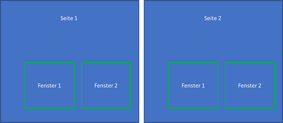
Die Anlage der Seiten und die Anordnung der Fenster findet nicht durch einen grafischen editor statt, sondern in Transaktion SE71. Hauptfenster ist ein fenstertype, es kann nur einmal in einem Formular vorkommen. Der Text werden über mehrere Seiten in einem Hauptfenster ausgegeben. Wenn das Fenster auf einer Seite vollständig mit Text und Daten gefüllt ist, wird der Text in einem Hauptfenster der folgeseite ausgegeben. In diesem Fall, erste Seite verweist auf die zweite Seite. Es kann auch sein, dass die Seite sich auf selbst verweist.
Konstantes Fenster: Es wird den Header und den Footer auf jeder Seite andruckt.
Rücksetzendes Fenster: Es wird immer in einer Seite zurückgesetzt und neu gefüllt werden. Beispielweise die Anzeige der Seitennummer.
Grafisches Fenster: In diesem Fenster, grafiken werden angezeigt.
Der Formularkopf enthält die Formatierung information wie z.b. Schriftart, Größe, einrückung, sprache, startseite, seitenlayout vor dem Druck, können Wir diese Information definieren.
Beispiel für Performance optimierten Code

- Wichtige Felder selektieren ( Select * vermeiden ).
DATA ls_corona TYPE corona.
SELECT person_id first_name FROM corona INTO ls_corona.
WRITE: / ls_corona-person_id, ls_corona-first_name.
ENDSELECT.
- Statt IF-Anweisung WHERE Clause nutzen.
SELECT person_id first_name FROM corona INTO ls_corona WHERE person_id = 100.
WRITE: / ls_corona-person_id, ls_corona-first_name.
ENDSELECT.
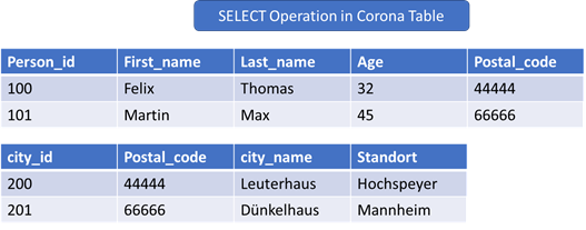
- Geschachtelter SELECTs vermeiden.
Beispiel für schlechten Code.
SELECT person_id FROM corona_table_1 INTO ls_corona_table_1.
SELECT city_id FROM corona_table_2 INTO ls_corona_table_2 WHERE postal_code = ls_corona_table_1-postal_code.
ENDSELECT.
ENDSELECT.
Beispiel für besseren Code.
SELECT person_id city_id FROM corona_table_1 INNER JOIN corona_table_2 ON
corona_table_1~postal_code = corona_table_2~postal_code.
ENDSELECT.
| Last auf dem Datenbankserver | Last auf dem Anwendungsserver |
| SELECT * FROM corona_table_1 INTO TABLE itab ORDER BY person_id | SELECT * FROM corona_table INTO TABLE itab. SORT itab by person_id. |