Python f-strings or formatted strings are new way of formatting strings introduced in Python 3.6 under PEP-498. It’s also called literal string interpolation. They provide a better way to format strings and make debugging easier too.
What are f-strings?
Strings in Python are usually enclosed in “ ” (double quotes) or ‘ ‘ ( single quotes). To create f-Strings, you only need to add an f or an F before the opening quotes of your string. For example,
“Anna” is a string whereas f”Anna” is an f-String.
f-Strings provide a concise and convenient way to embed python expressions inside string literals for formatting.
Why do we need f-Strings?
Before Python 2.6, to format a string, one would either use % operator or string.Template module. Later str.format method came along and added to the language a more flexible and robust way of formatting a string.
%formatting: great for simple formatting but limited support for strings, ints, doubles etc., We can’t use it with objects.
msg = ‘hello world’
‘msg: %s’ % msg
Output:
'msg: hello world'
Template strings:
Template strings are useful for keyword arguments like dictionaries. We cannot call any function and arguments must be string.
msg = ‘hello world’
‘msg: {}’.format(msg)
Output:
'msg: hello world'
String format():
String format() function was introduced to overcome the limitations of %formatting and template strings. But this also has verbosity.
age = 3 * 10
‘My age is {age}.’.format(age=age)
Output:
'My age is 30.'
Introduction of f-string in Python is to have minimal syntax for string formatting.
f-String Syntax:
f"This is an f-string {var_name} and {var_name}."
Enclosing of variables are within curly braces {}
Example:
val1 = ‘Abaython’
val2 = ‘Python’
print(f”{val1} is a portal for {val2}.”)
Output:
Abaython is a portal for Python.
How to evaluate expressions in f-String?
We can evaluate valid expressions on the fly using,
num1 = 25
num2 = 45
print(f”The product of {num1} and {num2} is {num1 * num2}.”)
You can think of one liner code as a block or segment of code compressed in one line to perform the similar function. This one liner saves you a lot of time, memory and you can also trick your friends or fellow programmers. It also keeps your program simple, clean, short and simple with less lines of code.
One need to be careful by using them, while Python is known for its ease of understanding and readability. You should keep in mind not to violate this feature.
Now let’s start!
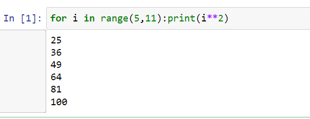
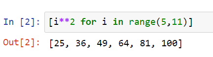
For loop in one line
If for loop is used in a list then use the below one.
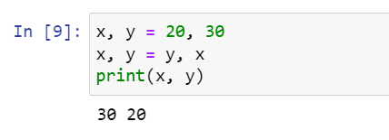
Swap variables
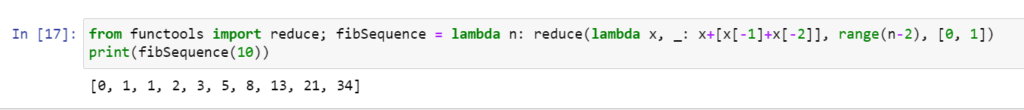
Fibonacci
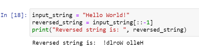
Reverse a string
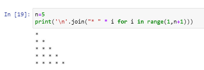
Print a pattern
These are some of the one liners in Python. Many more are there it’s always exciting while learning a new language to try these sorts of things. If you know any other one liners in Python leave your comment below.
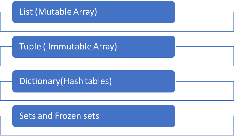
In Python we have 4 built-in data structures which covers 80% of the real-world data structures. These are classified as non-primitive data structures because they store a collection of values in various format than a single value. Some can store data structures within data structures, creating depth and complexity.
Built-in data structures are predefined data structures that come along with Python. Lists and tuples are ordered sequence of objects. Unlike strings that contain only characters, lists and tuples can contain any type of objects.
List and tuples are like arrays.
Tuples like strings are immutables.
Lists are mutables so they can be converted after their creation.
Sets are mutable unordered sequence of unique elements whereas frozensets are immutable sets
Lists are enclosed in brackets: l =[1,2,’a’]
Tuples are enclosed in parentheses: t=(1,2,’a’)
Dictionaries are built with curly brackets: d= {‘a’:1, ‘b’:2}
Set are built with curly brackets: s= {1,2,3}
Tuples are faster and consume less memory.
Lists:
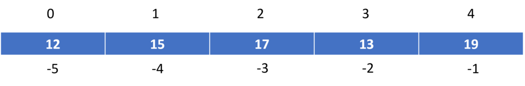
They are used to store data of different data types in a sequential manner. It stores heterogeneous data in sequential order. There are two types of indexing: positive index(most common method) and negative index.
Indexing:
Positive Index means every element has an index that starts from 0 and goes until last element.
Negative Index starts from -1 and it starts retrieving from last element.
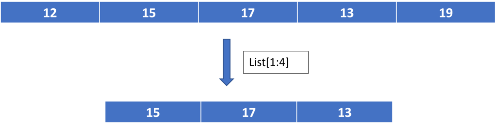
Slicing:
In Python List slicing is the most common practice to solve problems efficiently. If we want to use a range of elements from the list we can access those range with slicing and the operator used is colon (:)
Syntax:
List [start:end:index jump]
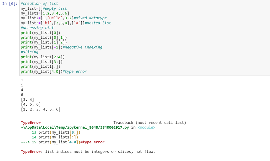
Type error occurs when data types other than integer are used to access like in our example float is used. Index error occurs when we try to access indexes out of range.
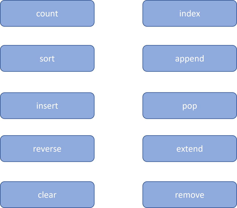
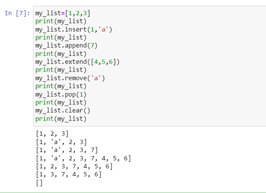
List Functions:
Let us see some functions in the sample code snippet:
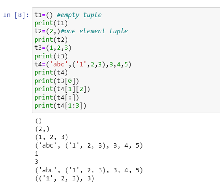
Tuple:
Tuples are same as list but the only exception is that data cannot be changed once entered into the tuple. They are immutable. Since it is immutable the length is fixed, to grow or shrink a tuple we need to create a new tuple. Like list tuple also has some methods
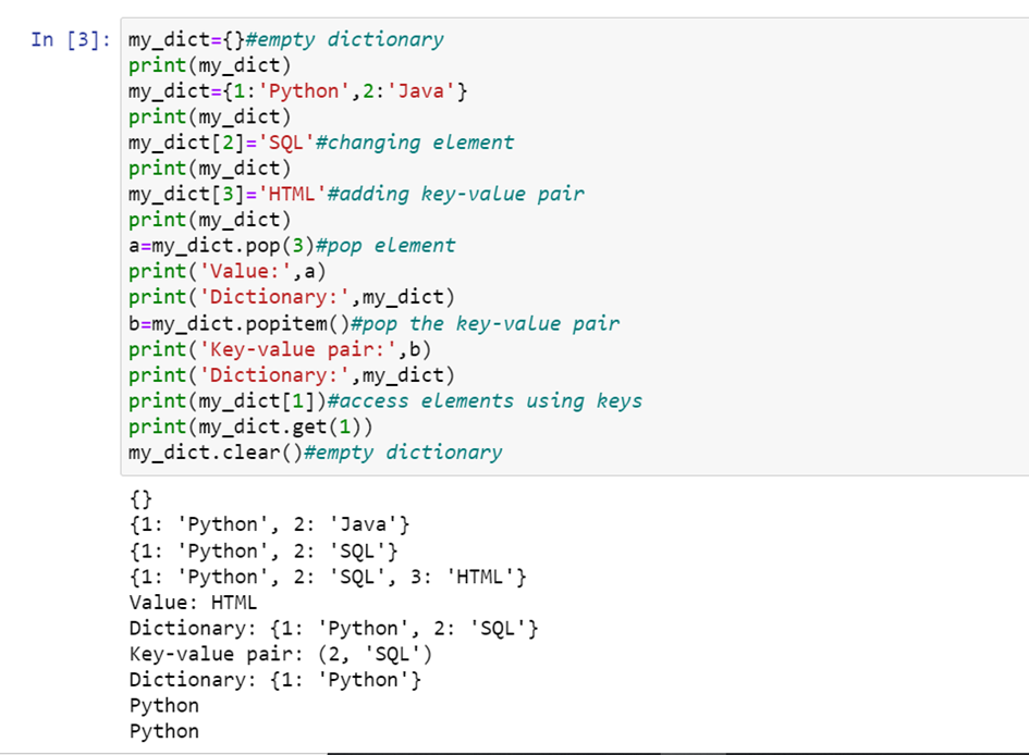
Dictionaries:
Dictionary is a datastructure which stores the data in the form of key:value pairs. Dictionary is a collection of ordered, changeable and does not allow duplication. Key-value is provided in dictionary to make it more optimized. For better understanding, dictionary can be compared to a telephone directory with tens of thousands of names and phone numbers. Here the constant values are names and phone numbers these are the keys and the various names and phone numbers fed to the keys are called values.
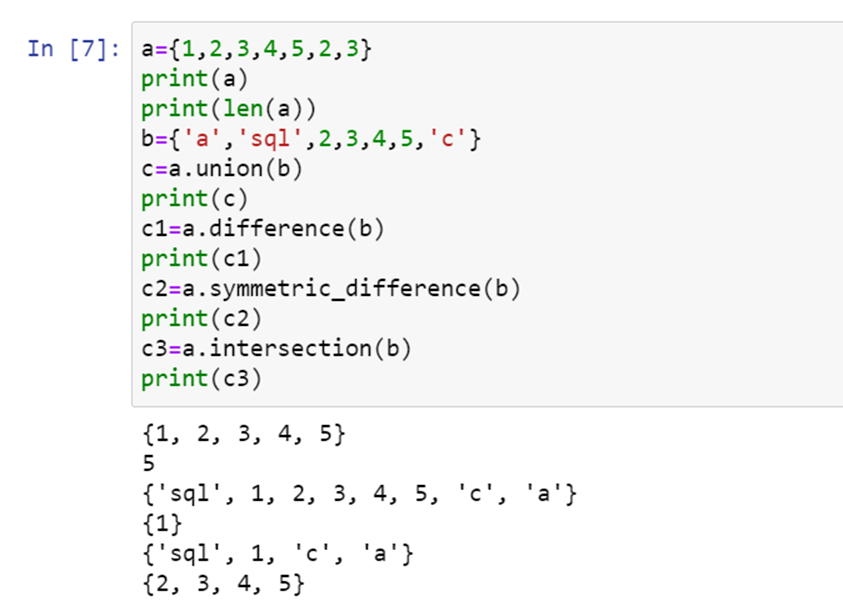
Sets:
Sets are a collection of unordered elements that are unique. Even if the data is repeated more than once it will be entered in the set only once. It is same as arithmetic sets.
Sets are created same way as in dictionary by using curly brackets but instead of key value pairs we pass values directly.
Now let us see a sample code snippet with set creation and its operations such as union, intersection, difference, symmetric_difference
Union combines both sets
Intersection finds the elements present in both sets
Difference deletes the elements present in both sets and outputs the elements present only in the set
Symmetric_difference is same as difference but outputs the data which is remaining in both sets.
These are all the four basic data structures one need to know while learning python programming.
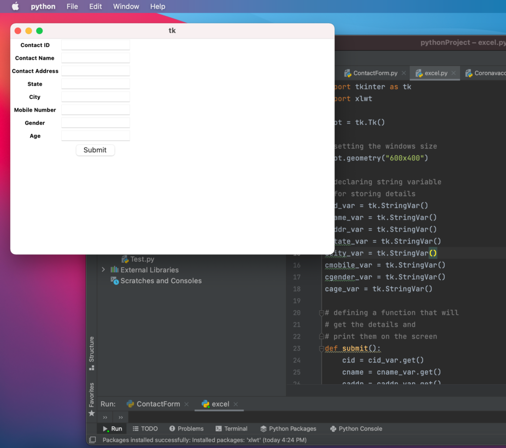
# defining a function that will # get the details and # print them on the screen def submit(): cid = cid_var.get() cname = cname_var.get() caddr = caddr_var.get() cstate = cstate_var.get() ccity = ccity_var.get() cmobile = cmobile_var.get() cgender = cgender_var.get() cage = cage_var.get()
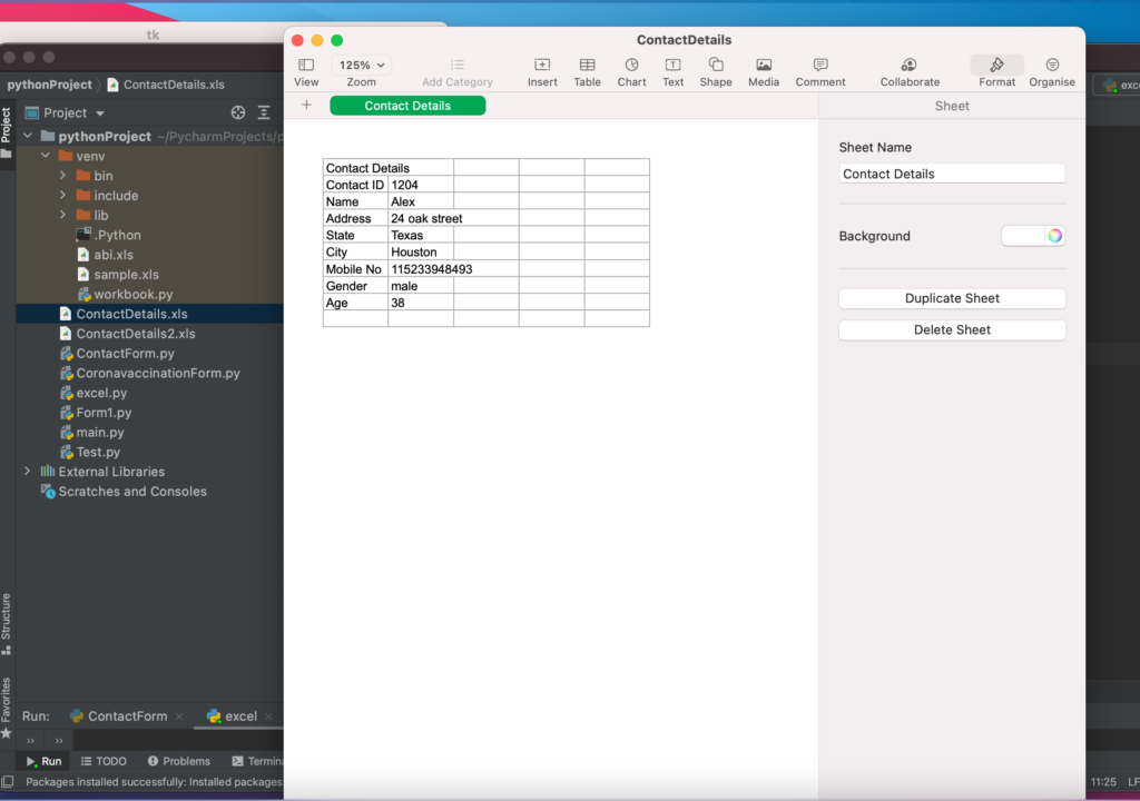
workbook = xlwt.Workbook()
#Naming the sheet in the excel sheet = workbook.add_sheet("Contact Details")
# performing an infinite loop # for the window to display root.mainloop()
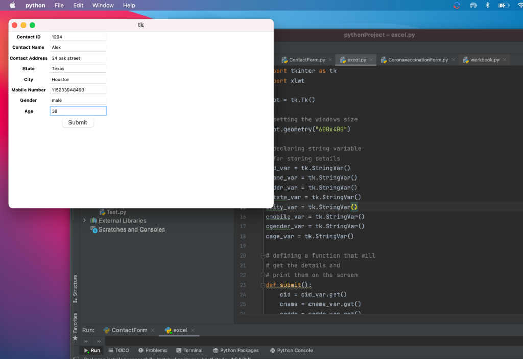
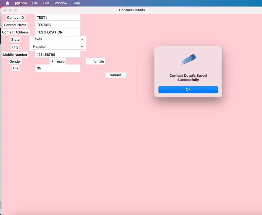
Upon running the program, the form will be displayedFeed the required form detailsAfter clicking submit, a excel will be generated where in all the given form data is stored
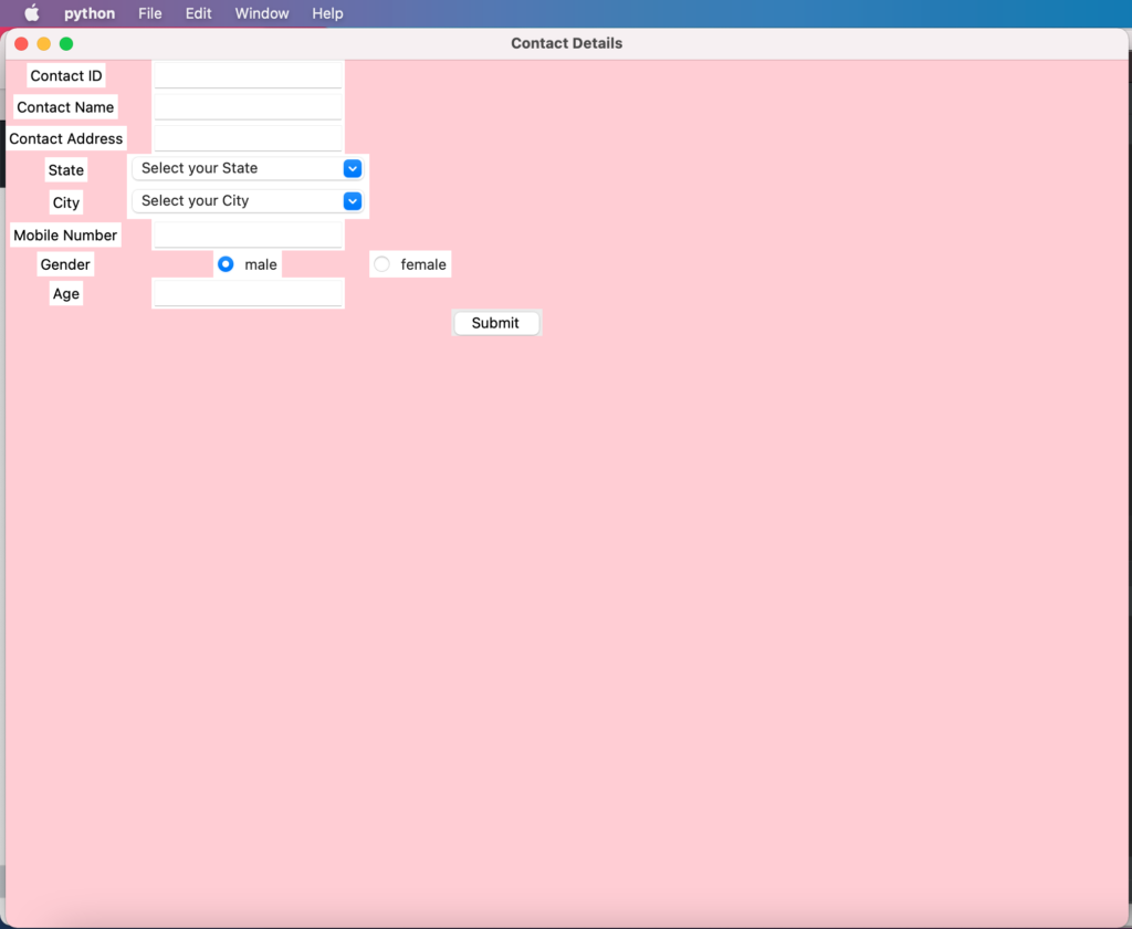
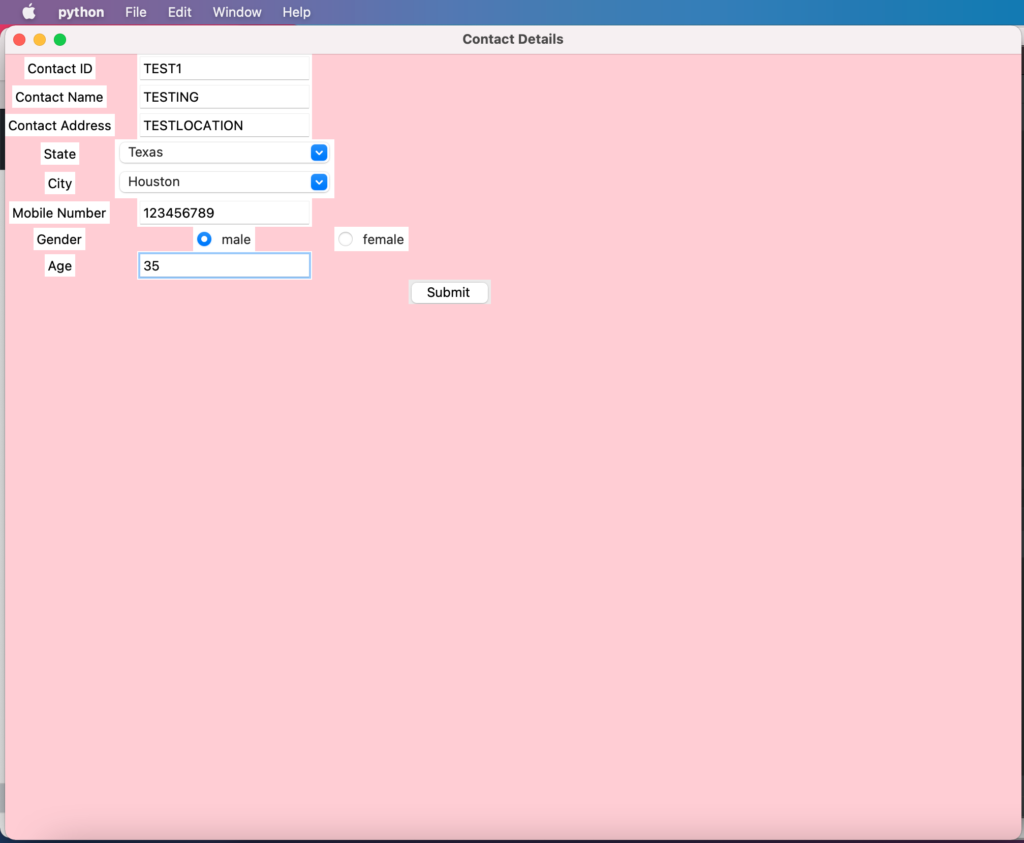
Tkinter is a python package that provides various controls, such as buttons, labels, radio buttons, text area and text boxes used in a GUI application. These controls are commonly called widgets. The Button widget is used to display buttons in your application.
Lets learn these UI controls via a simple form creation program:
from tkinter import * from tkinter import ttk from tkinter import messagebox
Run the program and form will get displayedUser should enter the required contact detailsUpon submitting the form, user will get the success response message
So far we have learned how to use TensorFlow to implement a basic neural network, going up all the way to a basic Convolutional Neural Network. In this article, we’ll go much further by taking the ideas we’ve learned and applied them to a much bigger dataset of cats versus dogs on Kaggle. Yes, so we take the full Kaggle dataset of 25,000 cats versus dogs images. So we want to take a look at what it’s like to train a much larger data set, and that was like a data science challenge, not that long ago. Now, we’re going to learn that here, which I think is really helpful to get great results while operating on much bigger data sets.
What does it take to download a public dataset of the Internet, like cats versus dogs, and get a neural network to work on it? Data is messy, sometimes you find astonishing things like pictures of people holding cats or multiple cats or surprising things in data. For example, you might have some files that are zero length and they could be corrupt as a result. So it’s like using your Python skills, using your TensorFlow skills to be able to filter them out. Building a convolutional neural network to be able to spot things like we mentioned, a person holding a cat. So that’s some of the things we need to concentrate on. We’ll be using a very clean dataset that we’re using with cats versus dogs, but you’re going to hit some of those issues. In this article, you’ll learn the skills that you need to be able to deal with other datasets that may not be as clean as this one.
The reality is, there’s a lot of data cleaning, and having great tools to help with that data cleaning makes our workflow much more efficient. Definitely, in this article, you will get to practice all that, as well as train a pretty cool neural network to classify cats versus dogs. Please go ahead.
In this article, we’ll take our understanding of the Convolutional Neural Network to the next level by recognizing sophisticated real images of Cats and Dogs in order to classify an incoming image as one or the other. In particular, the handwriting recognition made your life a little easier by having all the images be the same size and shape, and they were all monochrome color. Real-world images aren’t like that — they’re in different shapes, aspect ratios, etc, and they’re usually in color!
So, as part of the task you need to process your data — not least resizing it to be uniform in shape.
You’ll follow these steps:
Explore the Example Data of Cats and Dogs.
Build and train a Neural Network to recognize the difference between the two.
Evaluate Training and Validation accuracy.
Explore the Example Data
Let’s start by downloading our example data, a .zip of 2,000 JPG pictures of cats and dogs, and extracting it locally in /tmp.
NOTE: The 2,000 images used in this exercise are excerpted from the “Dogs vs. Cats” dataset available on Kaggle, which contains 25,000 images. Here, we use a subset of the full dataset to decrease training time.
The following python code will use the OS library to use Operating System libraries, giving you access to the file system, and the zip file library allowing you to unzip the data.
The contents of the .zip are extracted to the base directory /tmp/cats_and_dogs_filtered, which contains train and validation subdirectories for the training and validation datasets, which in turn each contain cats and dogs subdirectories.
In short: The training set is the data that is used to tell the neural network model that ‘this is what a cat looks like’, ‘this is what a dog looks like’ etc. The validation data set is images of cats and dogs that the neural network will not see as part of the training, so you can test how well or how badly it does in evaluating if an image contains a cat or a dog.
One thing to pay attention to in this sample: We do not explicitly label the images as cats or dogs. If you remember with the handwriting example earlier, we had labeled ‘this is a 1’, ‘this is a 7’ etc. Later you’ll see something called an ImageGenerator being used — and this is coded to read images from subdirectories, and automatically label them from the name of that subdirectory. So, for example, you will have a ‘training’ directory containing a ‘cats’ directory and a ‘dogs’ one. ImageGenerator will label the images appropriately for you, reducing a coding step.
We can find out the total number of cat and dog images in the train and validation directories:
print('total training cat images :', len(os.listdir(train_cats_dir)))
print('total training dog images :', len(os.listdir(train_dogs_dir)))

print('total validation cat images :', len(os.listdir(validation_cats_dir)))
print('total validation dog images :', len(os.listdir(validation_dogs_dir)))
For both cats and dogs, we have 1,000 training images and 500 validation images.
Now let’s take a look at a few pictures to get a better sense of what the cat and dog datasets look like. First, configure the matplot parameters:
%matplotlib inline

import matplotlib.image as mpimg
import matplotlib.pyplot as plt

# Parameters for our graph; we'll output images in a 4x4 configuration
nrows = 4
ncols = 4

pic_index = 0 # Index for iterating over images
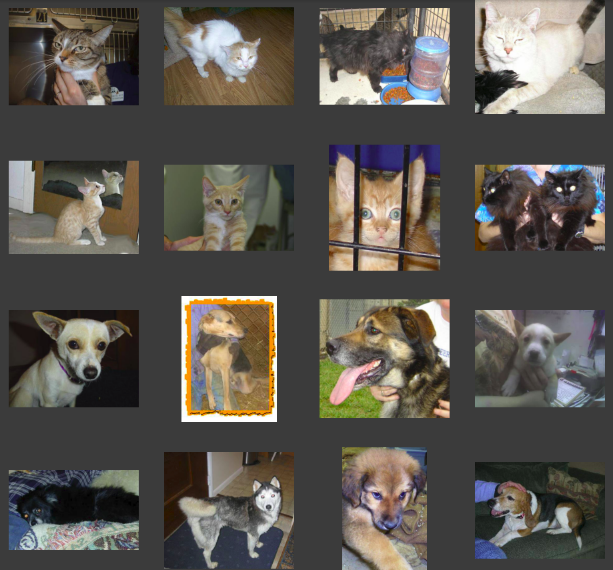
Now, display a batch of 8 cat and 8 dog pictures. You can rerun the cell to see a fresh batch each time:
# Set up matplotlib fig, and size it to fit 4x4 pics
fig = plt.gcf()
fig.set_size_inches(ncols*4, nrows*4)

pic_index+=8

next_cat_pix = [os.path.join(train_cats_dir, fname)
                for fname in train_cat_fnames[ pic_index-8:pic_index]
               ]

next_dog_pix = [os.path.join(train_dogs_dir, fname)
                for fname in train_dog_fnames[ pic_index-8:pic_index]
               ]

for i, img_path in enumerate(next_cat_pix+next_dog_pix):
  # Set up subplot; subplot indices start at 1
  sp = plt.subplot(nrows, ncols, i + 1)
  sp.axis('Off') # Don't show axes (or gridlines)

  img = mpimg.imread(img_path)
  plt.imshow(img)

plt.show()
Batch of 8 dogs and 8 cats.
It may not be obvious from looking at the images in this grid, but important note here, and a significant difference is that these images come in all shapes and sizes. These are color and in a variety of shapes. Before training a Neural network with them you’ll need to tweak the images. You’ll see that in the next section.
Ok, now that you have an idea of what your data looks like, the next step is to define the model that will be trained to recognize cats or dogs from these images
Building a Small Model from Scratch to Get to ~72% Accuracy
In the previous section, you saw that the images were in a variety of shapes and sizes. In order to train a neural network to handle them, you’ll need them to be in a uniform size. We’ve chosen 150×150 for this, and you’ll see the code that preprocesses the images to that shape shortly.
But before we continue, let’s start defining the model:
Step 1 will be to import tensorflow
Next, we will define a Sequential layer as before, adding some convolutional layers first. Note the input shape parameter this time. In the earlier example, it was 28x28x1, because the image was 28×28 in greyscale (8 bits, 1 byte for color depth). This time it is 150×150 for the size and 3 (24 bits, 3 bytes) for the color depth.
We then add a couple of convolutional layers as in the previous example and flatten the final result to feed into the densely connected layers.
Finally we add the densely connected layers.
Note that because we are facing a two-class classification problem, i.e. a binary classification problem, we will end our network with a sigmoid activation, so that the output of our network will be a single scalar between 0 and 1, encoding the probability that the current image is class 1 (as opposed to class 0).
model = tf.keras.models.Sequential([
    # Note the input shape is the desired size of the image 150x150 with 3 bytes color
    tf.keras.layers.Conv2D(16, (3,3), activation='relu', input_shape=(150, 150, 3)),
    tf.keras.layers.MaxPooling2D(2,2),
    tf.keras.layers.Conv2D(32, (3,3), activation='relu'),
    tf.keras.layers.MaxPooling2D(2,2),
    tf.keras.layers.Conv2D(64, (3,3), activation='relu'),
    tf.keras.layers.MaxPooling2D(2,2),
    # Flatten the results to feed into a DNN
    tf.keras.layers.Flatten(),
    # 512 neuron hidden layer
    tf.keras.layers.Dense(512, activation='relu'),
    # Only 1 output neuron. It will contain a value from 0-1 where 0 for 1 class ('cats') and 1 for the other ('dogs')
    tf.keras.layers.Dense(1, activation='sigmoid')
])
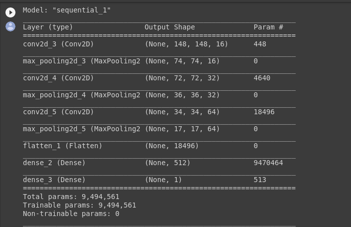
The model.summary() method call prints a summary of the NN
model.summary()
The “output shape” column shows how the size of your feature map evolves in each successive layer. The convolution layers reduce the size of the feature maps by a bit due to padding, and each pooling layer halves the dimensions.
Next, we’ll configure the specifications for model training. We will train our model with the loss because it’s a binary classification problem and our final activation is a sigmoid. We will use the rmsprop optimizer with a learning rate of 0.001. During training, we will want to monitor classification accuracy.
NOTE: In this case, using the RMSprop optimization algorithm is preferable to stochastic gradient descent (SGD), because RMSprop automates learning-rate tuning for us. (Other optimizers, such as Adam and Adagrad, also automatically adapt the learning rate during training, and would work equally well here.)
from tensorflow.keras.optimizers import RMSprop

model.compile(optimizer=RMSprop(lr=0.001),
              loss='binary_crossentropy',
              metrics = ['accuracy'])
Data Preprocessing
Let’s set up data generators that will read pictures in our source folders, convert them to tensors, and feed them (with their labels) to our network. We’ll have one generator for the training images and one for the validation images. Our generators will yield batches of 20 images of size 150×150 and their labels (binary).
As you may already know, data that goes into neural networks should usually be normalized in some way to make it more amenable to processing by the network. (It is uncommon to feed raw pixels into a convent.) In our case, we will preprocess our images by normalizing the pixel values to be in the [0, 1] range (originally all values are in the [0, 255] range).
In Keras, this can be done via the keras.preprocessing.image.ImageDataGenerator class using the rescale parameter. This ImageDataGenerator the class allows you to instantiate generators of augmented image batches (and their labels) via .flow(data, labels) or .flow_from_directory(directory). These generators can then be used with the Keras model methods that accept data generators as inputs: fit, evaluate_generator, and predict_generator.
from tensorflow.keras.preprocessing.image import ImageDataGenerator

# All images will be rescaled by 1./255.
train_datagen = ImageDataGenerator( rescale = 1.0/255. )
test_datagen  = ImageDataGenerator( rescale = 1.0/255. )

# --------------------
# Flow training images in batches of 20 using train_datagen generator
# --------------------
train_generator = train_datagen.flow_from_directory(train_dir,
                                                    batch_size=20,
                                                    class_mode='binary',
                                                    target_size=(150, 150))
# --------------------
# Flow validation images in batches of 20 using test_datagen generator
# --------------------
validation_generator =  test_datagen.flow_from_directory(validation_dir,
                                                         batch_size=20,
                                                         class_mode  = 'binary',
                                                         target_size = (150, 150))
Training
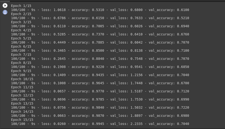
Let’s train on all 2,000 images available, for 15 epochs, and validate on all 1,000 test images.
Do note the values per epoch.
You’ll see 4 values per epoch — Loss, Accuracy, Validation Loss and Validation Accuracy.
Loss and Accuracy are a great indication of the progress of training. It’s making a guess as to the classification of the training data, and then measuring it against the known label, calculating the result. Accuracy is the portion of correct guesses. The Validation accuracy is the measurement with the data that has not been used in training. As expected this would be a bit lower. You’ll learn about why this occurs in the section on overfitting later in this course.
history = model.fit(train_generator,
                              validation_data=validation_generator,
                              steps_per_epoch=100,
                              epochs=15,
                              validation_steps=50,
                              verbose=2)
Evaluating Accuracy and Loss for the Model
Let’s plot the training/validation accuracy and loss as collected during training:
#-----------------------------------------------------------
# Retrieve a list of list results on training and test data
# sets for each training epoch
#-----------------------------------------------------------
acc = history.history[ 'accuracy' ]
val_acc = history.history[ 'val_accuracy' ]
loss = history.history[ 'loss' ]
val_loss = history.history['val_loss' ]
epochs = range(len(acc)) # Get number of epochs
#------------------------------------------------
# Plot training and validation accuracy per epoch
#------------------------------------------------
plt.plot ( epochs, acc )
plt.plot ( epochs, val_acc )
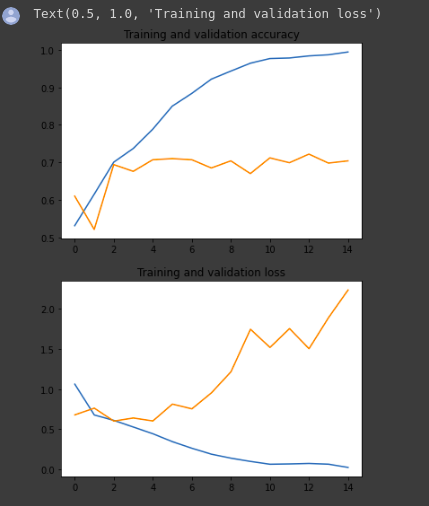
plt.title ('Training and validation accuracy')
plt.figure()
#------------------------------------------------
# Plot training and validation loss per epoch
#------------------------------------------------
plt.plot ( epochs, loss )
plt.plot ( epochs, val_loss )
plt.title ('Training and validation loss' )
As you can see, we are overfitting like it’s getting out of fashion. Our training accuracy (in blue) gets close to 100% (!) while our validation accuracy (in green) stalls as 70%. Our validation loss reaches its minimum after only five epochs.
Since we have a relatively small number of training examples (2000), overfitting should be our number one concern. Overfitting happens when a model exposed to too few examples learns patterns that do not generalize to new data, i.e. when the model starts using irrelevant features for making predictions. For instance, if you, as a human, only see three images of people who are lumberjacks, and three images of people who are sailors, and among them, the only person wearing a cap is a lumberjack, you might start thinking that wearing a cap is a sign of being a lumberjack as opposed to a sailor. You would then make a pretty lousy lumberjack/sailor classifier.
Overfitting is the central problem in machine learning: given that we are fitting the parameters of our model to a given dataset, how can we make sure that the representations learned by the model will be applied to data never seen before? How do we avoid learning things that are specific to the training data?
In the next exercise, we’ll look at ways to prevent overfitting in the cat vs. dog classification model.
Before going to discuss how computer identifies and labels objects let’s understand what is computer vision in detail.
“Computer vision is the field of having a computer understand and label what is present in an image(i.e, this is a dog or cat without being explicitly programmed) and then figure out the patterns.”
You can interpret what a shirt is or what a shoe is, but how would you program for that? if an extra terrestrial who had never seen clothing walked into the room with you, how would you explain the shoes to him? It’s really difficult, if not impossible to do right? And it’s the same problem with computer vision.
So one way to solve that is to use lots of pictures of clothing and tell the computer what that’s a picture of and then have the computer figure out the patterns that give you the difference between a shoe, and a shirt, and a handbag, and a coat.
For example, take a computer vision problem? Let’s take a look at a scenario where we can recognize different items of clothing, trained from a data set containing 10 different types.
Fashion-MNIST is available as a data set with an API call in TensorFlow(Tensorflow has in-built data sets available for learning purposes we just need to import them) but before that let’s start with our import of TensorFlow.
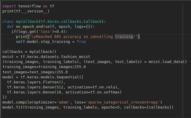
import tensorflow as tf
print(tf.__version__)
The Fashion MNIST data is available directly in the tf.keras datasets API. You load it like below.
mnist = tf.keras.datasets.fashion_mnist
In the MNIST data set, 60,000 of the 70,000 images are used to train the network, and then 10,000 images, one that it hasn’t previously seen, can be used to test just how good or how bad it is performing.
Calling load_data on this object will give you two sets of two lists, these will be the training and testing values for the graphics that contain the clothing items and their labels.
What do these values look like? Let’s print a training image, and a training label to see…Experiment with different indices in the array. For example, also take a look at index 0.
import numpy as np
np.set_printoptions(linewidth=200)
import matplotlib.pyplot as plt
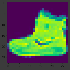
plt.imshow(training_images[0])
print(training_labels[0])
print(training_images[0])
If you notice that all of the values in the number are between 0 and 255. If we are training a neural network, for various reasons it’s easier if we treat all values as between 0 and 1, a process called ‘normalizing‘…and fortunately in Python it’s easy to normalize a list like this without looping.
Now you might be wondering why there are 2 sets…training and testing — remember the idea is to have 1 set of data for training, and then another set of data for testing…that the model hasn’t yet seen…to see how good it would be at classifying values. After all, when you’re done, you’re going to want to try it out with data that it hadn’t previously seen!
Let’s now design the model. There are quite a few new concepts here but don’t worry, you’ll get the hang of them by reading the description below.
model = tf.keras.models.Sequential([tf.keras.layers.Flatten(),
                                    tf.keras.layers.Dense(128, activation=tf.nn.relu),
                                    tf.keras.layers.Dense(10, activation=tf.nn.softmax)])
Sequential: That defines a SEQUENCE of layers in the neural network.
Flatten: Remember earlier where our images were a square when you printed them out? Flatten just takes that square and turns it into a 1-dimensional set.
Dense: Adds a layer of neurons.
Each layer of neurons needs an activation function to tell them what to do. There are lots of options, but just use these for now.
Relu effectively means “If X>0 return X, else return 0” — so what it does it only passes values 0 or greater to the next layer in the network.
Softmax takes a set of values, and effectively picks the biggest one, so, for example, if the output of the last layer looks like [0.1, 0.1, 0.05, 0.1, 9.5, 0.1, 0.05, 0.05, 0.05], it saves you from fishing through it looking for the biggest value, and turns it into [0,0,0,0,1,0,0,0,0] — The goal is to save a lot of coding! as well as time.
The next thing to do, now the model is defined, is to actually build it. You do this by compiling it with an optimizer and loss function as before — and then you train it by calling *model.fit * asking it to fit your training data to your training labels — i.e. have it figure out the relationship between the training data and its actual labels, so in future, if you have data that looks like the training data, then it can make a prediction for what that data would look like.
model.compile(optimizer = tf.optimizers.Adam(),
loss = 'sparse_categorical_crossentropy',
metrics=['accuracy'])
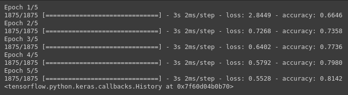
model.fit(training_images, training_labels, epochs=5)
Once it’s done training — you should see an accuracy value at the end of the final epoch. It might look something like 0.8142. This tells you that your neural network is about 81% accurate in classifying the training data. I.E., it figured out a pattern match between the image and the labels that worked 81% of the time. Not great, but not bad considering it was only trained for 5 epochs and done quite quickly.
But how would it work with unseen data? That’s why we have the test images.
We can call the function model.evaluate, and pass in the two sets, and it will report back the loss for each. Let’s take a look.
model.evaluate(test_images, test_labels)
An accuracy that was returned was about .7971, which means it was about 79% accurate. As expected it probably would not do as well with unseen data as it did with data it was trained on! As we move further, there are ways to improve this.
To explore further, let’s create a set of classifications for each of the test images, and then prints the first entry in the classifications.
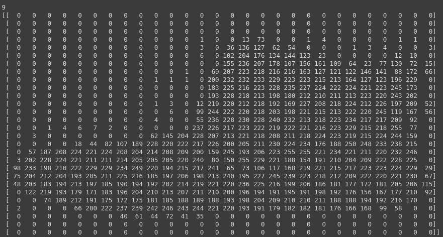
The output of the model is a list of 10 numbers. These numbers are a probability that the value being classified is the corresponding value, i.e., the first value in the list is the probability that the image is of a ‘0’ (T-shirt/top), the next is a ‘1’ (Trouser), etc. Notice that they are all VERY LOW probabilities.
For the 9 (Ankle boot), the probability was in the ’90s, i.e. the neural network is telling us that it’s almost certainly a 7. The 10th element on the list is the biggest, and the ankle boot is labeled 9. The list has the 10th element being the highest value means that the Neural Network has predicted that the item it is classifying is most likely an ankle boot.
We came to the end, so far we have loaded data, built a model, and fed with training data we predicted ankle boot. A few key points to consider are:
Increase the number of neurons — The impact is training takes longer but results are accurate. By adding more Neurons we have to do more calculations, slowing down the process, but in this case, they have a good impact — we do get more accurate. That doesn’t mean it’s always a case of ‘more is better’, you can hit the law of diminishing returns very quickly!
Remove the Flatten() layer. Why do you think that’s the case you get an error about the shape of the data. It may seem vague right now, but it reinforces the rule of thumb that the first layer in your network should be the same shape as your data. Right now our data is 28×28 images, and 28 layers of 28 neurons would be infeasible, so it makes more sense to ‘flatten’ that 28,28 into a 784×1. Instead of writing all the code to handle that ourselves, we add the Flatten() layer at the beginning, and when the arrays are loaded into the model later, they’ll automatically be flattened for us.
Change final (output) layers — You get an error as soon as it finds an unexpected value. Another rule of thumb — the number of neurons in the last layer should match the number of classes you are classifying for. In this case, it’s the digits 0-9, so there are 10 of them, hence you should have 10 neurons in your final layer.
Consider the effects of additional layers in the network — There isn’t a significant impact — because this is relatively simple data. For far more complex data (including color images to be classified as flowers), extra layers are often necessary.
The impact of training for more or fewer epochs — you might see the loss value stops decreasing, and sometimes increases. This is a side effect of something called ‘over-fitting’ and you need to keep an eye out for when training neural networks. There’s no point in wasting your time training if you aren’t improving your loss, right!
Callbacks — stop the training when I reach the desired value?’ — i.e. 95% accuracy might be enough for you, and if you reach that after 3 epochs, why sit around waiting for it to finish a lot more epochs…So how would you fix that? Like any other program…you have callbacks! Let’s see them in action…
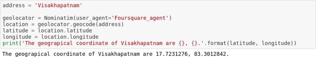
Visakhapatnam also known as Vizag, is the largest city in the Indian state of Andhra Pradesh and headquarters of the Visakhapatnam district and one of the four smart cities of Andhra Pradesh. In addition having great history, Vizag also have adorable climate for being situated between the Eastern Ghats and the coast of the Bay of Bengal which makes Vizag a tourism destination for many tourists for leisure activities.
The target audience for this project are tourists, helping them to explore the city to find out what are popular venues and cityscapes such as Neighbourhoods and Landmarks on their own instead of reaching out to a travel guide which puts additional cost in their budget.
Data
This section includes description of the data and how it will be used to solve the problem.
Clearly, to solve the above business problem we need location data. What is location data? Location data is data which describes places and venues, such as their geographical location, their category, working hours, full address, and so on, such that for a given location given in the form of its geographical coordinates (or latitude and longitude values) one is able to determine what types of venues exist within a defined radius from that location.
So, for a given location you will be able to tell which place exists nearby, it may be any place which is present in the data. The location data providers are i)Foursquare, ii)Google Places, iii)Yelp.
The best way to choose a Location data providers by considering these factors:
1)Rate Limits, 2)Costs, 3)Coverage, 4)Accuracy, 5)Update Frequency. Foursquare update their data continuously, whereas other providers would update their data either daily or weekly depending on their location data.
Data Collection:
Foursquare:
But as far as this project is concerned, we will use the Foursquare location data set since their data set to be the most comprehensive so far.Also creating a developer account to use their API is quite straightforward and easiest compared to other providers. We’ll explore the so called city by leveraging location data to find out the venues.
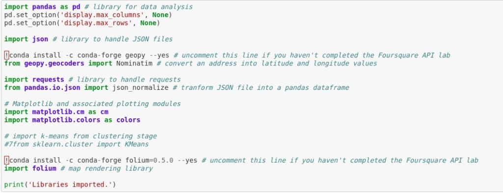
Web Scraping:
To extract the Cityscapes i.e., Neighbourhoods and Landmarks we’ll use BeautifulSoup package a Python library for getting data out of HTML, XML, and other markup languages.
Methodology
Methodology section represents the main component of the report where we’ll identify and explore the venues and display those venues with their respective addresses, upto 10 km as well as we’ll display the Neighbourhoods and Landmarks of Visakhapatnam city.
This would enable any visitor/tourist to identify the venues he/she wants to visit on their taste.
As a first step, we will retrieve the data from Foursquare API. We extract venue information from the center of Visakhapatnam, within 10 Km range.
Next, we’ll display places where venues are located and cityscapes so that any visitor can go to any place and enjoy the option to explore many venues and places on his/her own without the need of reaching out for a tourist guide.
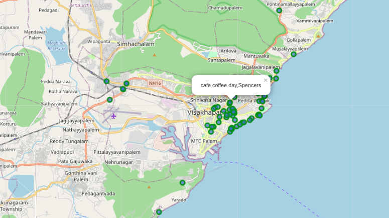
Finally, we’ll impose Venues and cityscapes on the Visakhapatnam map.
We’ll perform exploratory data analysis to find out the popular restaurants and category of the restaurants.
Before we start with the main content, let’s download all the dependencies that we will need.
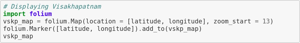
We begin by displaying geographical coordinates of the Visakhapatnam by using geocoder and nominatim to convert an address to it’s respective latitude and longitude.
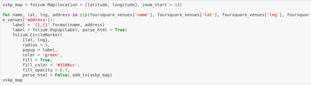
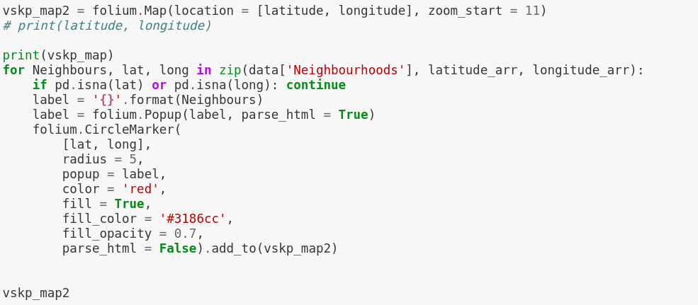
We can examine the Visakhapatnam map using Folium: a map rendering library which will impose Venues and address on top of it.
This piece of code works to show the Visakhapatnam map
Foursquare API:
We will fetch all venues in Visakhapatnam upto a range of 10 Kilometers from the center of the city using the Foursquare API. The Foursquare API has the explore API which allows us to find venue recommendations within a given radius for the given coordinates. We will use this API to find all the venues.
In order to access Foursquare data through API call we need to get an account. For this project we used developer account which is free of cost.
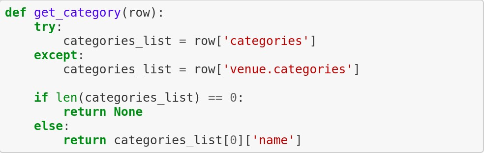
Function: get_category() to extract category names of the venues, as we know data we’ll be in the form of keys.
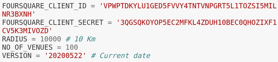
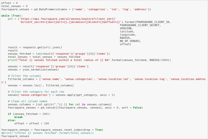
This block of code is common whenever we access Foursquare data through api calls.
We’ll call the API over and over till we get all venues within the given distance. The maximum venues this API can fetch is 100, so we will fetch all venues by iteratively calling this API and increasing the offset each time.
Foursquare API requires client_id, and client_secret to function which can be accessed by creating a developer account. We will set the radius as 10 Kilometers. The version is a required parameter which defines the date on which we are browsing so that it retrieves the latest data.
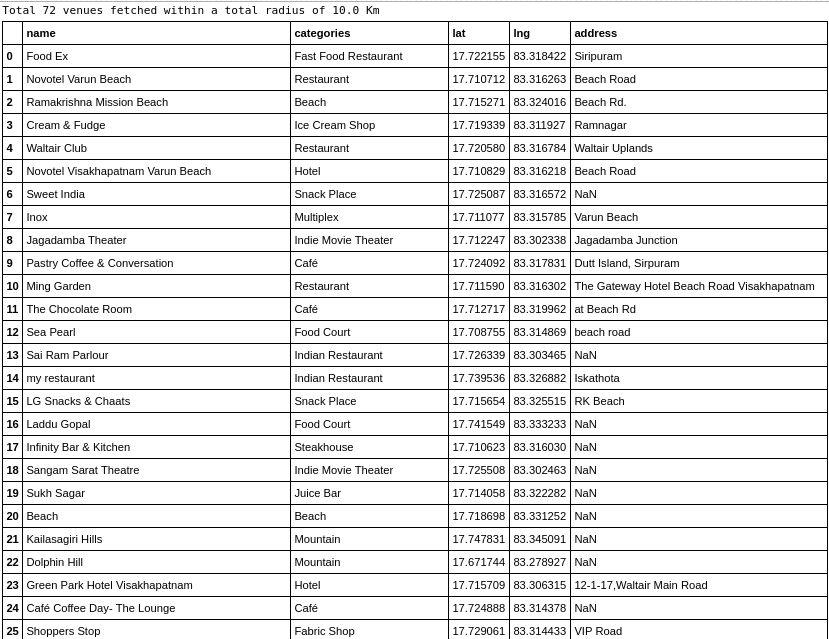
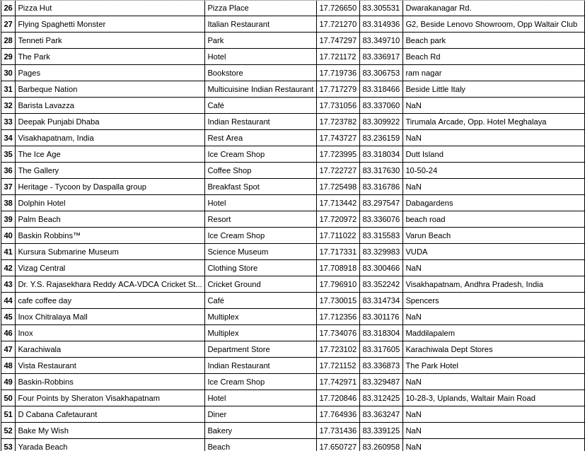
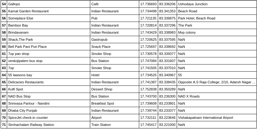
Venues fetched are:
Let’s visualize these Foursquare data items on the Visakhapatnam map.
Exploratory Data Analysis:
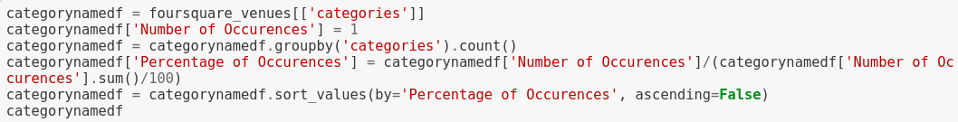
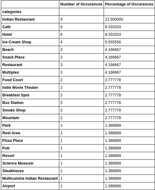
By using the Foursquare API we obtained information of the closest venues to the location coordinates which were provided. The information about these venues were then stored in a data frame Pandas a Python data analysis tool kit. The next stage of data analysis involves grouping these venues into categories and then determining what were the most and least prevalent types of venues in the Visakhapatnam city.
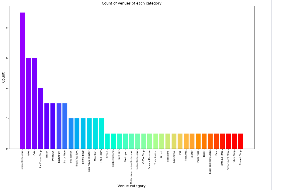
We will get what are the different categories of venues exists with their respective count.
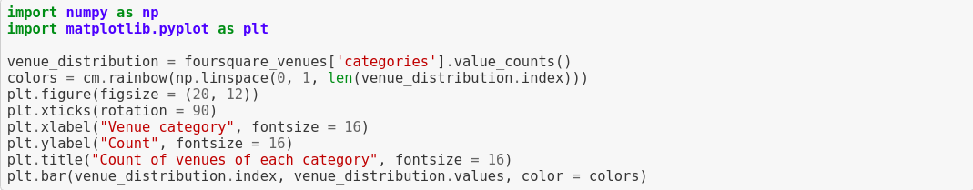
Let’s create a bar plot:
It’s evident that Indian restaurants are more popular in Visakhapatnam, tourists must make a preference to visit Indian restaurant to experience the gustatory delights of Indian cuisine. From the above table and graph they can decide which venue to visit and which one not to visit.
Web Scraping: Beautiful Soup
To understand simply, say you’vefound some webpages that display data relevant to you but that do not provide any way of downloading the data directly. Beautiful Soup helps you pull particular content from a webpage, remove the HTML markup, and save the information.
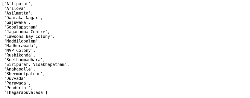
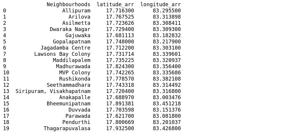
Neighbourhoods: Allipuram, Arilova, Asilmetta, Dwaraka Nagar, Gajuwaka, Gopalapatnam, Jagadamba Centre, Lawsons Bay Colony, Maddilapalem, Madhurawada, MVP Colony,Rushikonda,Seethammadhara, Siripuram, Visakhapatnam,Anakapalle,Bheemunipatnam,Duvvada,Parawada,Pendurthi, Thagarapuvalasa.
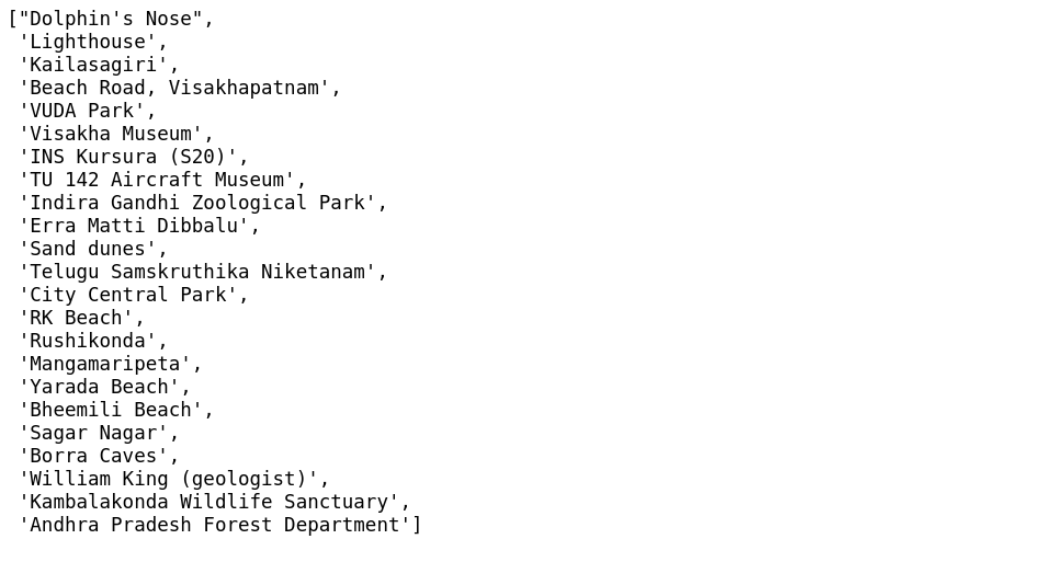
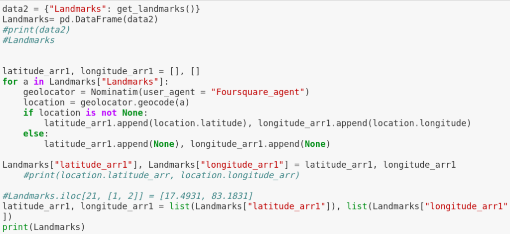
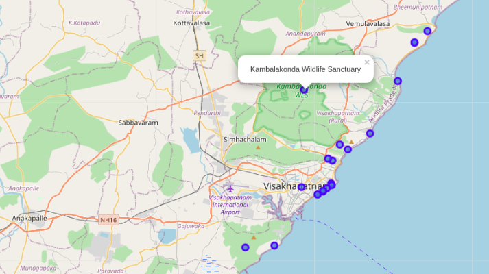
Landmarks: Dolphin’s Nose, Lighthouse, Kailasagiri, Beach Road, Visakhapatnam, VUDAPark,Visakha Museum, INS Kursura (S20), TU 142 Aircraft Museum, Indira Gandhi ZoologicalPark,Erra Matti Dibbalu, Sand dunes,TeluguSamskruthika Niketanam, City CentralPark,RK Beach,Rushikonda,Mangamaripeta,YaradaBeach, Bheemili Beach, Sagar Nagar, Borra Caves, William King (geologist), Kambalakonda Wildlife Sanctuary, Andhra PradeshForestDepartment.
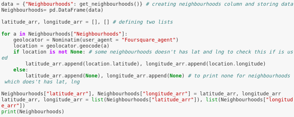
To display theseattractions on to the Visakhapatnam map we don’t have latitude and longitude readily available. So, we’ll be using geopy.geocoder and Nominatim to convert these addresses into latitude and longitude coordinates and then we’ll pass these coordinates in to folium to impose these places on to the Vizag map which we have done earlier in this project.
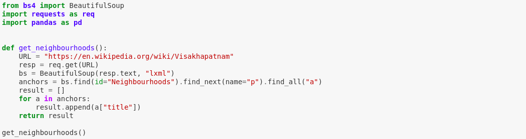
get_neighbourhoods() function: extracts all the anchor tags in the neighbourhood section from the wikipedia page
We have retrieved all the neighbours of vizag city.
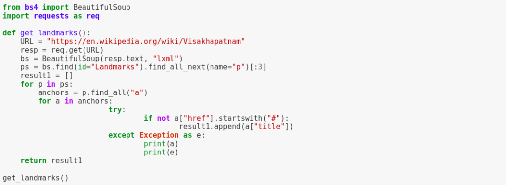
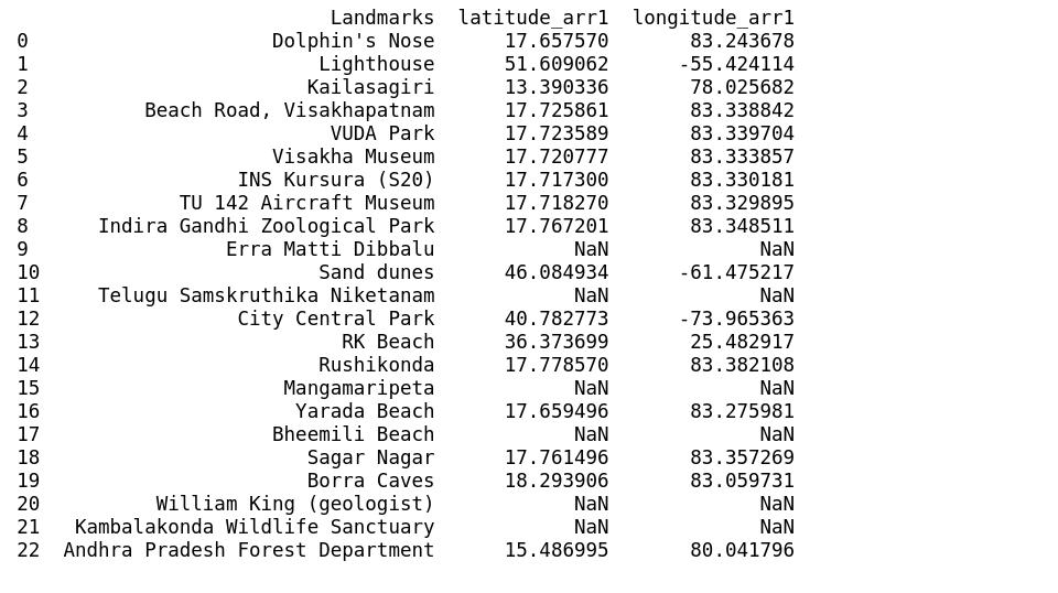
get_landmarks() function will extracts all the anchor tags in landmarks section:
Actually there are three paragraphs in Landmarks section and each section has citations. A citation is the way you tell your readers that certain material in your work came from another source. It also gives readers the information necessary to find that source again, including: information about the author, the title of the work.
While doing so parser is unable to parse through the code so, that’s why the try and except block is used to catch and handle exceptions. Python executes code following the try statement as a“normal”part of the program (we are taking title of the anchor tag). The code that follows the except statement is the program’s response to any exceptions in the preceding try clause.
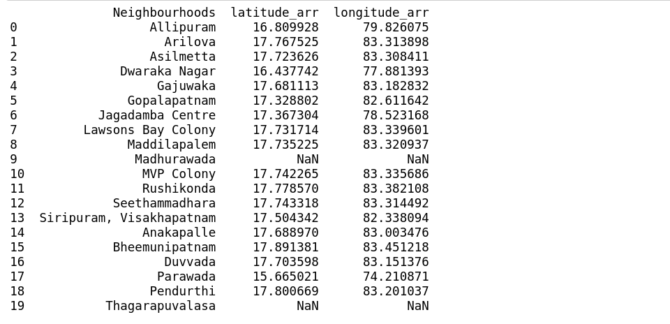
Let’s call get_neighbourhoods() function and store in Neighbourhoods data frame and pass it to geo locator to get the geographical coordinates.
Visakhapatnam latitudes start with ’17’ and longitudes start with ’83’.
As we can see it doesn’t satisfy above criteria and also has NaN values this may be for a variety of reasons like same place name exists in some other area and also maybe foursquare doesn’t have these data.
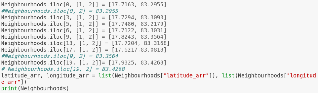
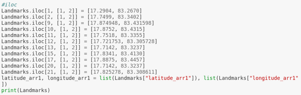
Using iloc method to correct the false data.
iloc gets rows (or columns) at particular positions in the index (so it only takes integers).
Neighbourhoods of Visakhapatnamalong with lat and lng.
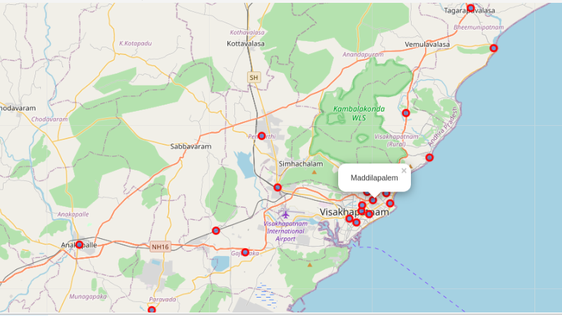
Map displaying Neighbourhoods
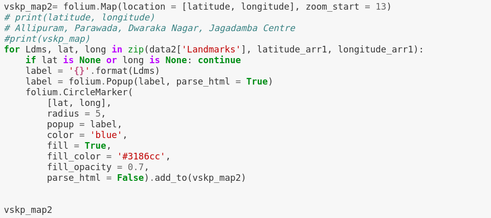
We have wide variety of options in choosing the colour of the marker as well as the size of the marker by simply adjusting the parameters.
Let’s call get_landmarks() function to extract all the landmarks.
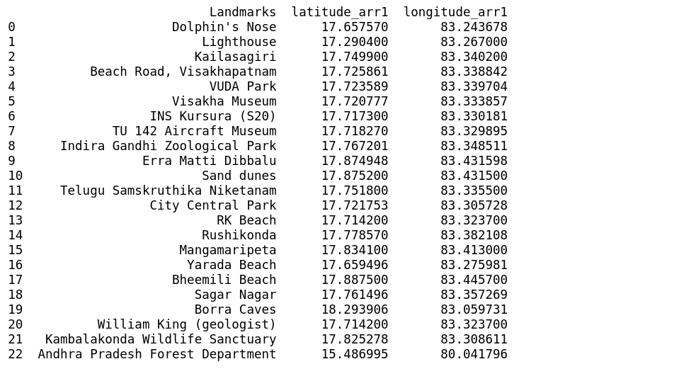
Entering latitude and longitude manually into the rows where data is not true by using iloc[] method
Landmarks of Visakhapatnam.
Results and Discussions:
Based on our analysis above, we can draw a number of conclusions that will be useful to aid any visitor visiting the city of Visakhapatnam, India.
After collecting data from the Foursquare, we got a list of 72 different venues. We identified that from the total set of venues, majority of them were Indian Restaurants. A visitor who loves Indian food would surely like to visit Visakhapatnam.
Finally,through clusters we identified that there are many venues which are clustered around’Varunbeach’, ‘Rk beach’, ‘Siripuram’, ‘SampathVinayakatemple’, ‘MVP colony’, ‘Diamond park’, ‘Beach road’.
On the other hand, we have visualized Neighbourhoods and Landmarks. Interestingly, most of the Landmarks are scattered at the beach corridor.
If you’re looking for Indian restaurants to taste Indian food Visakhapatnam can serve wide array of varieties to enjoy the food.
Conclusion:
The purpose of this project was to explore the places that a person visiting Visakhapatnam could visit. The venues have been identified using Foursquare and have been plotted on the map along with that Neighbourhoods and Landmarks also plotted. The map reveals that there are seven major areas a person can visit: Varun beach, RK beach, Siripuram, Sampath Vinayaka temple, MVP colony, Diamond park and Beach road. Based on the visitor’s reachability, he/she can choose amongst the places. If a touristor visits beach corrider more likely will cover up many places to be visited including popular venues also including landmarks.